


| Documentation: | Census 1990 on 2010 Geographies |
you are here:
choose a survey
survey
document
chapter
Publisher: U.S. Census Bureau
Survey: Census 1990 on 2010 Geographies
| Document: | Summary Tape File 3 |
| citation: | Social Explorer, U.S. Census Bureau; Census of Population and Housing, 1990: Summary Tape File 3 on CD-ROM [machine-readable data files] / prepared by the Bureau of the Census. Washington: The Bureau [producer and distributor], 1991. |
Chapter Contents
The data contained in this data product are based on the 1990 census sample. The data are estimates of the actual figures that would have been obtained from a complete count. Estimates derived from a sample are expected to be different from the 100-percent figures because they are subject to sampling and nonsampling errors. Sampling error in data arises from the selection of persons and housing units to be included in the sample. Nonsampling error affects both sample and 100-percent data, and is introduced as a result of errors that may occur during the collection and processing phases of the census. Provided below is a detailed discussion of both types of errors and a description of the estimation procedures.
Every person and housing unit in the United States was asked certain basic demographic and housing questions (for example, race, age, marital status, housing value, or rent). A sample of these persons and housing units was asked more detailed questions about such items as income, occupation, and housing costs in addition to the basic demographic and housing information. The primary sampling unit for the 1990 census was the housing unit, including all occupants. For persons living in group quarters, the sampling unit was the person. Persons in group quarters were sampled at a 1-in-6 rate.
The sample designation method depended on the data collection procedures. Approximately 95 percent of the population was enumerated by the mailback procedure. In these areas, the Bureau of the Census either purchased a commercial mailing list, which was updated by the United States Postal Service and Census Bureau field staff, or prepared a mailing list by canvassing and listing each address in the area prior to Census Day. These lists were computerized and the appropriate units were electronically designated as sample units. The questionnaires were either mailed or hand-delivered to the addresses with instructions to complete and mail back the form.
Housing units in governmental units with a precensus (1988) estimated population of fewer than 2,500 persons were sampled at 1-in-2. Governmental units were defined for sampling purposes as all incorporated places, all counties, all county equivalents such as parishes in Louisiana, and all minor civil divisions in Connecticut, Maine, Massachusetts, Michigan, Minnesota, New Hampshire, New Jersey, New York, Pennsylvania, Rhode Island, Vermont, and Wisconsin. Housing units in census tracts and block numbering areas (BNAs) with a precensus housing unit count below 2,000 housing units were sampled at 1-in-6 for those portions not in small governmental units (governmental units with a population less than 2,500). Housing units within census tracts and BNAs with 2,000 or more housing units were sampled at 1-in-8 for those portions not in small governmental units.
In list/enumerate areas (about 5 percent of the population), each enumerator was given a blank address register with designated sample lines. Beginning about Census Day, the enumerator systematically canvassed an assigned area and listed all housing units in the address register in the order they were encountered. Completed questionnaires, including sample information for any housing unit listed on a designated sample line, were collected. For all governmental units with fewer than 2,500 persons in list/enumerate areas, a 1-in-2 sampling rate was used. All other list/enumerate areas were sampled at 1-in-6.
Housing units in American Indian reservations, tribal jurisdiction statistical areas, and Alaska Native villages were sampled according to the same criteria as other governmental units, except the sampling rates were based on the size of the American Indian and Alaska Native population in those areas as measured in the 1980 census. Trust lands were sampled at the same rate as their associated American Indian reservations. Census designated places in Hawaii were sampled at the same rate as governmental units because the Census Bureau does not recognize incorporated places in Hawaii.
The purpose of using variable sampling rates was to provide relatively more reliable estimates for small areas and decrease respondent burden in more densely populated areas while maintaining data reliability. When all sampling rates were taken into account across the Nation, approximately one out of every six housing units in the Nation was included in the 1990 census sample.
To maintain the confidentiality required by law (Title 13, United States Code), the Bureau of the Census applies a confidentiality edit to the 1990 census data to assure that published data do not disclose information about specific individuals, households, or housing units. As a result, a small amount of uncertainty is introduced into the estimates of census characteristics. The sample itself provides adequate protection for most areas for which sample data are published since the resulting data are estimates of the actual counts; however, small areas require more protection. The edit is controlled so that the basic structure of the data is preserved.
The confidentiality edit is implemented by selecting a small subset of individual households from the internal sample data files and blanking a subset of the data items on these household records. Responses to those data items were then imputed using the same imputation procedures that were used for nonresponse. A larger subset of households is selected for the confidentiality edit for small areas to provide greater protection for these areas. The editing process is implemented in such a way that the quality and usefulness of the data were preserved.
The confidentiality edit is implemented by selecting a small subset of individual households from the internal sample data files and blanking a subset of the data items on these household records. Responses to those data items were then imputed using the same imputation procedures that were used for nonresponse. A larger subset of households is selected for the confidentiality edit for small areas to provide greater protection for these areas. The editing process is implemented in such a way that the quality and usefulness of the data were preserved.
Since statistics in this data product are based on a sample, they may differ somewhat from 100-percent figures that would have been obtained if all housing units, persons within those housing units, and persons living in group quarters had been enumerated using the same questionnaires, instructions, enumerators, etc. The sample estimate also would differ from other samples of housing units, persons within those housing units, and persons living in group quarters. The deviation of a sample estimate from the average of all possible samples is called the sampling error. The standard error of a sample estimate is a measure of the variation among the estimates from all the possible samples and thus is a measure of the precision with which an estimate from a particular sample approximates the average result of all possible samples. The sample estimate and its estimated standard error permit the construction of interval estimates with prescribed confidence that the interval includes the average result of all possible samples. Described below is the method of calculating standard errors and confidence intervals for the data in this product.
In addition to the variability which arises from the sampling procedures, both sample data and 100-percent data are subject to nonsampling error. Nonsampling error may be introduced during any of the various complex operations used to collect and process census data. For example, operations such as editing, reviewing, or handling questionnaires may introduce error into the data. A detailed discussion of the sources of nonsampling error is given in the section on Control of Nonsampling Error in this appendix.
Nonsampling error may affect the data in two ways. Errors that are introduced randomly will increase the variability of the data and should therefore be reflected in the standard error. Errors that tend to be consistent in one direction will make both sample and 100-percent data biased in that direction. For example, if respondents consistently tend to under-report their income, then the resulting counts of households or families by income category will tend to be understated for the higher income categories and overstated for the lower income categories. Such biases are not reflected in the standard error.
Tables A through C in this appendix contain the information necessary to calculate the standard errors of sample estimates in this data product. To calculate the standard error, it is necessary to know the basic standard error for the characteristic (given in table A or B) that would result under a simple random sample design (of persons, households, or housing units) and estimation technique; the design factor for the particular characteristic estimated (given in table C); and the number of persons or housing units in the tabulation area and the percent of these in the sample. For machine-readable products, the percent-in-sample is included in a data matrix on the file for each tabulation area. In printed reports, the percent-in-sample is provided in data tables at the end of the statistical tables that compose the report. The design factors reflect the effects of the actual sample design and complex ratio estimation procedure used for the 1990 census.
The steps given below should be used to calculate the standard error of an estimate of a total or a percentage contained in this product. A percentage is defined here as a ratio of a numerator to a denominator where the numerator is a subset of the denominator. For example, the proportion of Black teachers is the ratio of Black teachers to all teachers.
An illustration of the use of the tables is given in the section entitled Use of Tables to Compute Standard Errors.
The steps given below should be used to calculate the standard error of an estimate of a total or a percentage contained in this product. A percentage is defined here as a ratio of a numerator to a denominator where the numerator is a subset of the denominator. For example, the proportion of Black teachers is the ratio of Black teachers to all teachers.
- Obtain the standard error from table A or B (or use the formula given below the table) for the estimated total or percentage, respectively.
- Find the geographic area to which the estimate applies in the appropriate percent-in-sample table or appropriate matrix, and obtain the person or housing unit percent-in-sample figure for this area. Use the person percent-in-sample figure for person and family characteristics. Use the housing unit percent-in-sample figure for housing unit characteristics.
- Use table C to obtain the design factor for the characteristic (for example, employment status, school enrollment) and the range that contains the percentin- sample with which you are working. Multiply the basic standard error by this factor.
An illustration of the use of the tables is given in the section entitled Use of Tables to Compute Standard Errors.
The standard errors estimated from these tables are not directly applicable to sums of and differences between two sample estimates. To estimate the standard error of a sum or difference, the tables are to be used somewhat differently in the following three situations:
This method, however, will underestimate (overestimate) the standard error if the two items in a sum are highly positively (negatively) correlated or if the two items in a difference are highly negatively (positively) correlated. This method may also be used for the difference between (or sum of) sample estimates from two censuses or from a census sample and another survey. The standard error for estimates not based on the 1990 census sample must be obtained from an appropriate source outside of this appendix.
3. For the differences between two estimates, one of which is a subclass of the other, use the tables directly where the calculated difference is the estimate of interest. For example, to determine the estimate of non-Black teachers, one may subtract the estimate of Black teachers from the estimate of total teachers. To determine the standard error of the estimate of non-Black teachers apply the above formula directly.
- For the sum of or difference between a sample estimate and a 100-percent value, use the standard error of the sample estimate. The complete count value is not subject to sampling error.
- For the sum of or difference between two sample estimates, the appropriate standard error is approximately the square root of the sum of the two individual standard errors squared; that is, for standard errors:
This method, however, will underestimate (overestimate) the standard error if the two items in a sum are highly positively (negatively) correlated or if the two items in a difference are highly negatively (positively) correlated. This method may also be used for the difference between (or sum of) sample estimates from two censuses or from a census sample and another survey. The standard error for estimates not based on the 1990 census sample must be obtained from an appropriate source outside of this appendix.
3. For the differences between two estimates, one of which is a subclass of the other, use the tables directly where the calculated difference is the estimate of interest. For example, to determine the estimate of non-Black teachers, one may subtract the estimate of Black teachers from the estimate of total teachers. To determine the standard error of the estimate of non-Black teachers apply the above formula directly.
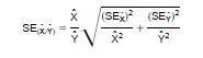
Frequently, the statistic of interest is the ratio of two variables, where the numerator is not a subset of the denominator. For example, the ratio of teachers to students in public elementary schools. The standard error of the ratio between two sample estimates is estimated as follows:
1. If the ratio is a proportion, then follow the procedure outlined for Totals and Percentages.
2. If the ratio is not a proportion, then approximate the standard error using the formula below.
1. If the ratio is a proportion, then follow the procedure outlined for Totals and Percentages.
2. If the ratio is not a proportion, then approximate the standard error using the formula below.
For the standard error of the median of a characteristic, it is necessary to examine the distribution from which the median is derived, as the size of the base and the distribution itself affect the standard error. An approximate method is given here. As the first step, compute one-half of the number on which the median is based (refer to this result as N/2). Treat N/2 as if it were an ordinary estimate and obtain its standard error as instructed above. Compute the desired confidence interval about N/2. Starting with the lowest value of the characteristic, cumulate the frequencies in each category of the characteristic until the sum equals or first exceeds the lower limit of the confidence interval about N/2. By linear interpolation, obtain a value of the characteristic corresponding to this sum. This is the lower limit of the confidence interval of the median. In a similar manner, continue cumulating frequencies until the sum equals or exceeds the count in excess of the upper limit of the interval about N/2. Interpolate as before to obtain the upper limit of the confidence interval for the estimated median.
When interpolation is required in the upper open-ended interval of a distribution to obtain a confidence bound, use 1.5 times the lower limit of the open-ended confidence interval as the upper limit of the open-ended interval.
When interpolation is required in the upper open-ended interval of a distribution to obtain a confidence bound, use 1.5 times the lower limit of the open-ended confidence interval as the upper limit of the open-ended interval.
A sample estimate and its estimated standard error may be used to construct confidence intervals about the estimate. These intervals are ranges that will contain the average value of the estimated characteristic that results over all possible samples, with a known probability. For example, if all possible samples that could result under the 1990 census sample design were independently selected and surveyed under the same conditions, and if the estimate and its estimated standard error were calculated for each of these samples, then:
1. Approximately 68 percent of the intervals from one estimated standard error below the estimate to one estimated standard error above the estimate would contain the average result from all possible samples;
2. Approximately 90 percent of the intervals from 1.645 times the estimated standard error below the estimate to 1.645 times the estimated standard error above the estimate would contain the average result from all possible samples.
3. Approximately 95 percent of the intervals from two estimated standard errors below the estimate to two estimated standard errors above the estimate would contain the average result from all possible samples.
The intervals are referred to as 68 percent, 90 percent, and 95 percent confidence intervals, respectively. The average value of the estimated characteristic that could be derived from all possible samples is or is not contained in any particular computed interval. Thus, we cannot make the statement that the average value has a certain probability of falling between the limits of the calculated confidence interval. Rather, one can say with a specified probability of confidence that the calculated confidence interval includes the average estimate from all possible samples (approximately the 100-percent value).
Confidence intervals also may be constructed for the ratio, sum of, or difference between two sample figures. This is done by first computing the ratio, sum, or difference, then obtaining the standard error of the ratio, sum, or difference (using the formulas given earlier), and finally forming a confidence interval for this estimated ratio, sum, or difference as above. One can then say with specified confidence that this interval includes the ratio, sum, or difference that would have been obtained by averaging the results from all possible samples.
The estimated standard errors given in this appendix do not include all portions of the variability due to nonsampling error that may be present in the data. The standard errors reflect the effect of simple response variance, but not the effect of correlated errors introduced by enumerators, coders, or other field or processing personnel. Thus, the standard errors calculated represent a lower bound of the total error. As a result, confidence intervals formed using these estimated standard errors may not meet the stated levels of confidence (i.e., 68, 90, or 95 percent). Thus, some care must be exercised in the interpretation of the data in this data product based on the estimated standard errors.
A standard sampling theory text should be helpful if the user needs more information about confidence intervals and nonsampling errors.
The following is a hypothetical example of how to compute a standard error of a total and a percentage. Suppose a particular data table shows that for City A 9,948 persons out of all 15,888 persons age 16 years and over were in the civilian labor force. The percent-in-sample table lists City A with a percent-in-sample of 16.0 percent (Persons column). The column in table C which includes 16.0 percent-in-sample shows the design factor to be 1.1 for Employment status.
The basic standard error for the estimated total 9,948 may be obtained from table A or from the formula given below table A. In order to avoid interpolation, the use of the formula will be demonstrated here. Suppose that the total population of City A was 21,220. The formula for the basic standard error, SE, is

The standard error of the estimated 9,948 persons 16 years and over who were in the civilian labor force is found by multiplying the basic standard error 163 by the design factor, 1.1 from table C. This yields an estimated standard error of 179 for the total number of persons 16 years and over in City A who were in the civilian labor force.
The estimated percent of persons 16 years and over who were in the civilian labor force in City A is 62.6. From table B, the unadjusted standard error is found to be approximately 0.85 percentage points. The standard error for the estimated 62.6 percent of persons 16 years and over who were in the civilian labor force is 0.85 x 1.1 = 0.94 percentage points.
A note of caution concerning numerical values is necessary. Standard errors of percentages derived in this manner are approximate. Calculations can be expressed to several decimal places, but to do so would indicate more precision in the data than is justifiable. Final results should contain no more than two decimal places when the estimated standard error is one percentage point (i.e., 1.00) or more.
In the previous example, the standard error of the 9,948 persons 16 years and over in City A who were in the civilian labor force was found to be 179. Thus, a 90 percent confidence interval for this estimated total is found to be:
[9.948 - 1.645(179)] to [9.948 + 1.645(179)] or 9.654 to 10.242
One can say, with about 90 percent confidence, that this interval includes the value that would have been obtained by averaging the results from all possible samples.
The following is an illustration of the calculation of standard errors and confidence intervals when a difference between two sample estimates is obtained. For example, suppose the number of persons in City B age 16 years and over who were in the civilian labor force was 9,314 and the total number of persons 16 years and over was 16,666. Further suppose the population of City B was 25,225. Thus, the estimated percentage of persons 16 years and over who were in the civilian labor force is 55.9 percent. The unadjusted standard error determined using the formula provided at the bottom of table B is 0.86 percentage points. We find that City B had a percent-in-sample of 15.7. The range which includes 15.7 percent-in-sample in table C shows the design factor to be 1.1 for Employment Status. Thus, the approximate standard error of the percentage (55.9 percent) is 0.86 x 1.1 = 0.95 percentage points.
Now suppose that one wished to obtain the standard error of the difference between City A and City B of the percentages of persons who were 16 years and over and who were in the civilian labor force. The difference in the percentages of interest for the two cities is:
62.6 - 55.9 = 6.7 percent.
Using the results of the previous example:

The 90 percent confidence interval for the difference is formed as before:
[6.70 - 1.645(134)] tp [6.70 + 1.645(1.34)] or 4.50 to 8.90
One can say with 90 percent confidence that the interval includes the difference that would have been obtained by averaging the results from all possible samples.
For reasonably large samples, ratio estimates are normally distributed, particularly for the census population. Therefore, if we can calculate the standard error of a ratio estimate then we can form a confidence interval around the ratio. Suppose that one wished to obtain the standard error of the ratio of the estimate of persons who were 16 years and over and who were in the civilian labor force in City A to the estimate of persons who were 16 years and over and who were in the civilian labor force in City B. The ratio of the two estimates of interest is:
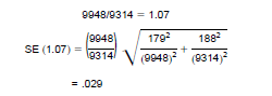
results above, the 90 percent confidence interval for this ratio would be:
[1.07 - 1.645(.029)] to [1.07 + 1.645(.029)] or 1.02 to 1.12
The basic standard error for the estimated total 9,948 may be obtained from table A or from the formula given below table A. In order to avoid interpolation, the use of the formula will be demonstrated here. Suppose that the total population of City A was 21,220. The formula for the basic standard error, SE, is
The standard error of the estimated 9,948 persons 16 years and over who were in the civilian labor force is found by multiplying the basic standard error 163 by the design factor, 1.1 from table C. This yields an estimated standard error of 179 for the total number of persons 16 years and over in City A who were in the civilian labor force.
The estimated percent of persons 16 years and over who were in the civilian labor force in City A is 62.6. From table B, the unadjusted standard error is found to be approximately 0.85 percentage points. The standard error for the estimated 62.6 percent of persons 16 years and over who were in the civilian labor force is 0.85 x 1.1 = 0.94 percentage points.
A note of caution concerning numerical values is necessary. Standard errors of percentages derived in this manner are approximate. Calculations can be expressed to several decimal places, but to do so would indicate more precision in the data than is justifiable. Final results should contain no more than two decimal places when the estimated standard error is one percentage point (i.e., 1.00) or more.
In the previous example, the standard error of the 9,948 persons 16 years and over in City A who were in the civilian labor force was found to be 179. Thus, a 90 percent confidence interval for this estimated total is found to be:
[9.948 - 1.645(179)] to [9.948 + 1.645(179)] or 9.654 to 10.242
One can say, with about 90 percent confidence, that this interval includes the value that would have been obtained by averaging the results from all possible samples.
The following is an illustration of the calculation of standard errors and confidence intervals when a difference between two sample estimates is obtained. For example, suppose the number of persons in City B age 16 years and over who were in the civilian labor force was 9,314 and the total number of persons 16 years and over was 16,666. Further suppose the population of City B was 25,225. Thus, the estimated percentage of persons 16 years and over who were in the civilian labor force is 55.9 percent. The unadjusted standard error determined using the formula provided at the bottom of table B is 0.86 percentage points. We find that City B had a percent-in-sample of 15.7. The range which includes 15.7 percent-in-sample in table C shows the design factor to be 1.1 for Employment Status. Thus, the approximate standard error of the percentage (55.9 percent) is 0.86 x 1.1 = 0.95 percentage points.
Now suppose that one wished to obtain the standard error of the difference between City A and City B of the percentages of persons who were 16 years and over and who were in the civilian labor force. The difference in the percentages of interest for the two cities is:
62.6 - 55.9 = 6.7 percent.
Using the results of the previous example:
The 90 percent confidence interval for the difference is formed as before:
[6.70 - 1.645(134)] tp [6.70 + 1.645(1.34)] or 4.50 to 8.90
One can say with 90 percent confidence that the interval includes the difference that would have been obtained by averaging the results from all possible samples.
For reasonably large samples, ratio estimates are normally distributed, particularly for the census population. Therefore, if we can calculate the standard error of a ratio estimate then we can form a confidence interval around the ratio. Suppose that one wished to obtain the standard error of the ratio of the estimate of persons who were 16 years and over and who were in the civilian labor force in City A to the estimate of persons who were 16 years and over and who were in the civilian labor force in City B. The ratio of the two estimates of interest is:
results above, the 90 percent confidence interval for this ratio would be:
[1.07 - 1.645(.029)] to [1.07 + 1.645(.029)] or 1.02 to 1.12
The estimates which appear in this publication were obtained from an iterative ratio estimation procedure (iterative proportional fitting) resulting in the assignment of a weight to each sample person or housing unit record. For any given tabulation area, a characteristic total was estimated by summing the weights assigned to the persons or housing units possessing the characteristic in the tabulation area. Estimates of family or household characteristics were based on the weight assigned to the family member designated as householder. Each sample person or housing unit record was assigned exactly one weight to be used to produce estimates of all characteristics. For example, if the weight given to a sample person or housing unit had the value 6, all characteristics of that person or housing unit would be tabulated with the weight of 6. The estimation procedure, however, did assign weights varying from person to person or housing unit to housing unit. The estimation procedure used to assign the weights was performed in geographically defined weighting areas. Weighting areas generally were formed of contiguous geographic units which agreed closely with census tabulation areas within counties. Weighting areas were required to have a minimum sample of 400 persons. Weighting areas never crossed State or county boundaries. In small counties with a sample count below 400 persons, the minimum required sample condition was relaxed to permit the entire county to become a weighting area.
Within a weighting area, the ratio estimation procedure for persons was performed in four stages. For persons, the first stage applied 17 household-type groups. The second stage used two groups: sampling rate of 1-in-2; sampling rate less than 1-in-2. The third stage used the dichotomy householders/nonhouseholders. The fourth stage applied 180 aggregate age-sex-race-Hispanic origin categories. The stages were as follows:
Within a weighting area, the first step in the estimation procedure was to assign an initial weight to each sample person record. This weight was approximately equal to the inverse of the probability of selecting a person for the census sample.
The next step in the estimation procedure, prior to iterative proportional fitting, was to combine categories in each of the four estimation stages, when needed to increase the reliability of the ratio estimation procedure. For each stage, any group that did not meet certain criteria for the unweighted sample count or for the ratio of the 100-percent to the initially weighted sample count, was combined, or collapsed, with another group in the same stage according to a specified collapsing pattern. At the fourth stage, an additional criterion concerning the number of complete count persons in each race/Hispanic origin category was applied.
As the final step, the initial weights underwent four stages of ratio adjustment applying the grouping procedures described above. At the first stage, the ratio of the complete census count to the sum of the initial weights for each sample person was computed for each stage I group. The initial weight assigned to each person in a group was then multiplied by the stage I group ratio to produce an adjusted weight.
In stage II, the stage I adjusted weights were again adjusted by the ratio of the complete census count to the sum of the stage I weights for sample persons in each stage II group. Next, at stage III, the stage II weights were adjusted by the ratio of the complete census count to the sum of the stage II weights for sample persons in each stage III group. Finally, at stage IV, the stage III weights were adjusted by the ratio of the complete census count to the sum of the stage III weights for sample persons in each stage IV group. The four stages of ratio adjustment were performed two times (two iterations) in the order given above. The weights obtained from the second iteration for stage IV were assigned to the sample person records. However, to avoid complications in rounding for tabulated data, only whole number weights were assigned. For example, if the final weight of the persons in a particular group was 7.25 then 1/4 of the sample persons in this group were randomly assigned a weight of 8, while the remaining 3/4 received a weight of 7.
The ratio estimation procedure for housing units was essentially the same as that for persons, except that vacant units were treated differently. The occupied housing unit ratio estimation procedure was done in four stages, and the vacant housing unit ratio estimation procedure was done in a single stage. The first stage for occupied housing units applied 16 household type categories, while the second stage used the two sampling categories described above for persons. The third stage applied three units-in-structure categories; i.e. single units, multi-unit less than 10 and multi-unit 10 or more. The fourth stage could potentially use 200 tenure-race-Hispanic origin-value/rent groups. The stages for ratio estimation for housing units were as follows:
The estimates produced by this procedure realize some of the gains in sampling efficiency that would have resulted if the population had been stratified into the ratio estimation groups before sampling, and if the sampling rate had been applied independently to each group. The net effect is a reduction in both the standard error and the possible bias of most estimated characteristics to levels below what would have resulted from simply using the initial, unadjusted weight. A by-product of this estimation procedure is that the estimates from the sample will, for the most part, be consistent with the complete count figures for the population and housing unit groups used in the estimation procedure.
Within a weighting area, the ratio estimation procedure for persons was performed in four stages. For persons, the first stage applied 17 household-type groups. The second stage used two groups: sampling rate of 1-in-2; sampling rate less than 1-in-2. The third stage used the dichotomy householders/nonhouseholders. The fourth stage applied 180 aggregate age-sex-race-Hispanic origin categories. The stages were as follows:
| PERSONS | |
|---|---|
| STAGE 1: TYPE OF HOUSEHOLD | |
| Group | Persons in Housing Units With a Family With Own Children Under 18 |
| 1 | 2 persons in housing unit |
| 2 | 3 persons in housing unit |
| 3 | 4 persons in housing unit |
| 4 | 5 to 7 persons in housing unit |
| 5 | 8 or more persons in housing unit |
| Persons in Housing Units With a Family Without Own Children Under 18 | |
| 6-10 | 2 through 8 or more persons in housing unit |
| Persons in All Other Housing Units | |
| 11 | 1 person in housing unit |
| 12-16 | 2 through 8 or more persons in housing unit |
| Persons in Group Quarters | |
| 17 | Persons in Group Quarters |
| STAGE II: SAMPLING RATES | |
| 1 | Sampling rate of 1-in-2 |
| 2 | Sampling rate less than 1-in-2 |
| STAGE Ill: HOUSEHOLDER/NONHOUSEHOLDER | |
| 1 | Householder |
| 2 | Nonhouseholder |
| STAGE IV: AGE/ SEX/ RACE/ HISPANIC ORIGIN | |
| Group | White |
| Persons of Hispanic Origin | |
| Male | |
| 1 | 0 to 4 years |
| 2 | 5 to 14 years |
| 3 | 15 to 19 year's |
| 4 | 20 to 24 years |
| 5 | 25 to 34 years |
| 6 | 35 to 54 year's |
| 7 | 55 to 64 years |
| 8 | 65 to 74 years |
| 9 | 75 years and over |
| Female | |
| 10-18 | Same age categories as groups 1 through 9. |
| Persons Not of Hispanic Origin | |
| 19-36 | Same sex and age categories as groups 1 through 18. |
| Black | |
| 37-72 | Same age/ sex/ Hispanic origin categories as groups 1 through 36. |
| Asian or Pacific Islander | |
| 73-108 | Same age/ sex/ Hispanic origin categories as groups 1 through 36. |
| American Indian, Eskimo, or Aleut | |
| 109-144 | Same age/ sex,/ Hispanic origin categories as groups 1 through 36. |
| Other Race (includes those races not listed above) | |
| 145-180 | Same age/ sex/ Hispanic origin categories as groups 1 through 36. |
Within a weighting area, the first step in the estimation procedure was to assign an initial weight to each sample person record. This weight was approximately equal to the inverse of the probability of selecting a person for the census sample.
The next step in the estimation procedure, prior to iterative proportional fitting, was to combine categories in each of the four estimation stages, when needed to increase the reliability of the ratio estimation procedure. For each stage, any group that did not meet certain criteria for the unweighted sample count or for the ratio of the 100-percent to the initially weighted sample count, was combined, or collapsed, with another group in the same stage according to a specified collapsing pattern. At the fourth stage, an additional criterion concerning the number of complete count persons in each race/Hispanic origin category was applied.
As the final step, the initial weights underwent four stages of ratio adjustment applying the grouping procedures described above. At the first stage, the ratio of the complete census count to the sum of the initial weights for each sample person was computed for each stage I group. The initial weight assigned to each person in a group was then multiplied by the stage I group ratio to produce an adjusted weight.
In stage II, the stage I adjusted weights were again adjusted by the ratio of the complete census count to the sum of the stage I weights for sample persons in each stage II group. Next, at stage III, the stage II weights were adjusted by the ratio of the complete census count to the sum of the stage II weights for sample persons in each stage III group. Finally, at stage IV, the stage III weights were adjusted by the ratio of the complete census count to the sum of the stage III weights for sample persons in each stage IV group. The four stages of ratio adjustment were performed two times (two iterations) in the order given above. The weights obtained from the second iteration for stage IV were assigned to the sample person records. However, to avoid complications in rounding for tabulated data, only whole number weights were assigned. For example, if the final weight of the persons in a particular group was 7.25 then 1/4 of the sample persons in this group were randomly assigned a weight of 8, while the remaining 3/4 received a weight of 7.
The ratio estimation procedure for housing units was essentially the same as that for persons, except that vacant units were treated differently. The occupied housing unit ratio estimation procedure was done in four stages, and the vacant housing unit ratio estimation procedure was done in a single stage. The first stage for occupied housing units applied 16 household type categories, while the second stage used the two sampling categories described above for persons. The third stage applied three units-in-structure categories; i.e. single units, multi-unit less than 10 and multi-unit 10 or more. The fourth stage could potentially use 200 tenure-race-Hispanic origin-value/rent groups. The stages for ratio estimation for housing units were as follows:
| OCCUPIED HOUSING UNITS | |
|---|---|
| STAGE 1: TYPE OF HOUSEHOLD | |
| Group | Housing Units With a Family With Own Children Under 18 |
| 1 | 2 persons in housing unit |
| 2 | 3 persons in housing unit |
| 3 | 4 persons in housing unit |
| 4 | 5 to 7 persons in housing unit |
| 5 | 8 or more persons in housing unit |
| Housing Units With a Family Without Own Children Under 18 | |
| 6-10 | 2 through 8 or more persons in housing unit |
| All Other Housing Units | |
| 11 | 1 person in housing unit |
| 12-16 | 2 through 8 or more persons in housing unit |
| STAGE II: SAMPLING RATE CATEGORY | |
| 1 | Sampling rate of 1-in-2 |
| 2 | Sampling rate less than 1-in-2 |
| STAGE III: UNITS IN STRUCTURE | |
| 1 | Single unit structure |
| 2 | Multi-unit structure consisting of fewer than 10 individual units |
| 3 | Multi-unit structure consisting of 10 or more individual units |
| STAGE IV: TENURE/ RACE AND HISPANIC ORIGIN OF HOUSEHOLDER/VALUE OR RENT | |
| Group | Owner |
| White Householder | |
| Householder of Hispanic Origin | |
| Value | |
| 1 | Less than $20,000 |
| 2 | $20,000 to $39,999 |
| 3 | $40,000 to $59,999 |
| 4 | $60,000 to $79,999 |
| 5 | $80,000 to $99,999 |
| 6 | $100,000 to $149,999 |
| 7 | $150,000 to $249,999 |
| 8 | $250,000 to $299,999 |
| 9 | $300,000 or more |
| 10 | Other[1] |
| Householder Not of Hispanic Origin | |
| 11-20 | Same value categories as groups 1 through 10 |
| Black Householder | |
| 21-40 | Same Hispanic origin/value categories as groups 1 through 20 |
| Asian or Pacific Islander Householder | |
| 41-60 | Same Hispanic origin/value categories as groups 1 through 20 |
| American Indian, Eskimo, or Aleut Householder | |
| 61-80 | Same Hispanic origin/value categories as groups 1 through 20 |
| Householder of Other Race | |
| 81-100 | Same Hispanic origin/value categories as groups 1 through 20 |
| Renter | |
| White Householder | |
| Householder of Hispanic origin | |
| Rent | |
| 101 | Less than $100 |
| 102 | $100 to $199 |
| 103 | $200 to $299 |
| 104 | $300 to $399 |
| 105 | $400 to $499 |
| 106 | $500 to $599 |
| 107 | $600 to $749 |
| 108 | $750 to $999 |
| 109 | $1,000 or more |
| 110 | No cash rent |
| Householder Not of Hispanic Origin | |
| 111-120 | Same rent categories as groups 101 through 110 |
| Black Householder | |
| 121-140 | Same Hispanic origin/rent categories as groups 101 through 120 |
| Asian or Pacific Islander Householder | |
| 141-160 | Same Hispanic origin/ rent categories as groups 101 through 120 |
| American Indian, Eskimo, or Aleut Householder | |
| 161-180 | Same Hispanic origin/ rent categories as groups 101 through 120 |
| Householder of Other Race | |
| 181-200 | Same Hispanic origin/ rent categories as groups 101 through 120 |
| Vacant Housing Units | |
| 1 | Vacant for rent |
| 2 | Vacant for sale |
| 3 | Other vacant |
| [1] | Value of units in this category results from other factors besides housing value alone, for example, inclusion of more than 10 acres of land,or presence of a business establishment on the premises. |
The estimates produced by this procedure realize some of the gains in sampling efficiency that would have resulted if the population had been stratified into the ratio estimation groups before sampling, and if the sampling rate had been applied independently to each group. The net effect is a reduction in both the standard error and the possible bias of most estimated characteristics to levels below what would have resulted from simply using the initial, unadjusted weight. A by-product of this estimation procedure is that the estimates from the sample will, for the most part, be consistent with the complete count figures for the population and housing unit groups used in the estimation procedure.
As mentioned earlier, both sample and 100-percent data are subject to nonsampling error. This component of error could introduce serious bias into the data, and the total error could increase dramatically over that which would result purely from sampling. While it is impossible to completely eliminate nonsampling error from an operation as large and complex as the decennial census, the Bureau of the Census attempted to control the sources of such error during the collection and processing operations. Described below are the primary sources of nonsampling error and the programs instituted for control of this error. The success of these programs, however, was contingent upon how well the instructions actually were carried out during the census. As part of the 1990 census evaluation program, both the effects of these programs and the amount of error remaining after their application will be evaluated.
It is possible for some households or persons to be missed entirely by the census. The undercoverage of persons and housing units can introduce biases into the data.
Several coverage improvement programs were implemented during the development of the census address list and census enumeration and processing to minimize undercoverage of the population and housing units. These programs were developed based on experience from the 1980 census and results from the 1990 census testing cycle. In developing and updating the census address list, the Census Bureau used a variety of specialized procedures in different parts of the country.
More extensive discussion of the programs implemented to improve coverage will be published by the Census Bureau when the evaluation of the coverage improvement program is completed.
Several coverage improvement programs were implemented during the development of the census address list and census enumeration and processing to minimize undercoverage of the population and housing units. These programs were developed based on experience from the 1980 census and results from the 1990 census testing cycle. In developing and updating the census address list, the Census Bureau used a variety of specialized procedures in different parts of the country.
- In the large urban areas, the Census Bureau purchased and geocoded address lists. Concurrent with geocoding, the United States Postal Service (USPS) reviewed and updated this list. After the postal check, census enumerators conducted a dependent canvass and update operation. In the fall of 1989, local officials were given the opportunity to examine block counts of address listings (local review) and identify possible errors. Prior to mailout, the USPS conducted a final review.
- In small cities, suburban areas, and selected rural parts of the country, the Census Bureau created the address list through a listing operation. The USPS reviewed and updated this list, and the Census Bureau reconciled USPS corrections and updated through a field operation. In the fall of 1989, local officials participated in reviewing block counts of address listings. Prior to mailout, the USPS conducted a final review.
- The Census Bureau (rather than the USPS) conducted a listing operation in the fall of 1989 and delivered census questionnaires in selected rural and seasonal housing areas in March of 1990. In some inner-city public housing developments, whose addresses had been obtained via the purchased address list noted above, census questionnaires were also delivered by Census Bureau enumerators.
More extensive discussion of the programs implemented to improve coverage will be published by the Census Bureau when the evaluation of the coverage improvement program is completed.
The person answering the questionnaire or responding to the questions posed by an enumerator could serve as a source of error, although the questions were phrased as clearly as possible based on precensus tests, and detailed instructions for completing the questionnaire were provided to each household. In addition, respondents answers were edited for completeness and consistency, and problems were followed up as necessary.
The enumerator may misinterpret or otherwise incorrectly record information given by a respondent; may fail to collect some of the information for a person or household; or may collect data for households that were not designated as part of the sample. To control these problems, the work of enumerators was monitored carefully. Field staff were prepared for their tasks by using standardized training packages that included hands-on experience in using census materials. A sample of the households interviewed by enumerators for nonresponse were reinterviewed to control for the possibility of data for fabricated persons being submitted by enumerators. Also, the estimation procedure was designed to control for biases that would result from the collection of data from households not designated for the sample.
The enumerator may misinterpret or otherwise incorrectly record information given by a respondent; may fail to collect some of the information for a person or household; or may collect data for households that were not designated as part of the sample. To control these problems, the work of enumerators was monitored carefully. Field staff were prepared for their tasks by using standardized training packages that included hands-on experience in using census materials. A sample of the households interviewed by enumerators for nonresponse were reinterviewed to control for the possibility of data for fabricated persons being submitted by enumerators. Also, the estimation procedure was designed to control for biases that would result from the collection of data from households not designated for the sample.
The many phases involved in processing the census data represent potential sources for the introduction of nonsampling error. The processing of the census questionnaires includes the field editing, followup, and transmittal of completed questionnaires; the manual coding of write-in responses; and the electronic data processing. The various field, coding and computer operations undergo a number of quality control checks to insure their accurate application.
Nonresponse to particular questions on the census questionnaire allows for the introduction of bias into the data, since the characteristics of the nonrespondents have not been observed and may differ from those reported by respondents. As a result, any imputation procedure using respondent data may not completely reflect this difference either at the elemental level (individual person or housing unit) or on the average. Some protection against the introduction of large biases is afforded by minimizing nonresponse. In the census, nonresponse was reduced substantially during the field operations by the various edit and followup operations aimed at obtaining a response for every question. Characteristics for the nonresponses remaining after this operation were imputed by the computer by using reported data for a person or housing unit with similar characteristics.
The objective of the processing operation is to produce a set of data that describes the population as accurately and clearly as possible. To meet this objective, questionnaires were edited during field data collection operations for consistency, completeness, and acceptability. Questionnaires also were reviewed by census clerks for omissions, certain specific inconsistencies, and population coverage. For example, write-in entries such as Dont know or NA were considered unacceptable. For some district offices, the initial edit was automated; however, for the majority of the district offices, it was performed by clerks. As a result of this operation, a telephone or personal visit followup was made to obtain missing information. Potential coverage errors were included in the followup, as well as a sample of questionnaires with omissions and/or inconsistencies. Subsequent to field operations, remaining incomplete or inconsistent information on the questionnaires was assigned using imputation procedures during the final automated edit of the collected data. Imputations, or computer assignments of acceptable codes in place of unacceptable entries or blanks, are needed most often when an entry for a given item is lacking or when the information reported for a person or housing unit on that item is inconsistent with other information for that same person or housing unit. As in previous censuses, the general procedure for changing unacceptable entries was to assign an entry for a person or housing unit that was consistent with entries for persons or housing units with similar characteristics. The assignment of acceptable codes in place of blanks or unacceptable entries enhances the usefulness of the data.
Another way in which corrections were made during the computer editing process was through substitution; that is, the assignment of a full set of characteristics for a person or housing unit. When there was an indication that a housing unit was occupied but the questionnaire contained no information for the people within the household or the occupants were not listed on the questionnaire, a previously accepted household was selected as a substitute, and the full set of characteristics for the substitute was duplicated. The assignment of the full set of housing characteristics occurred when there was no housing information available. If the housing unit was determined to be occupied, the housing characteristics were assigned from a previously processed occupied unit. If the housing unit was vacant, the housing characteristics were assigned from a previously processed vacant unit.
Another way in which corrections were made during the computer editing process was through substitution; that is, the assignment of a full set of characteristics for a person or housing unit. When there was an indication that a housing unit was occupied but the questionnaire contained no information for the people within the household or the occupants were not listed on the questionnaire, a previously accepted household was selected as a substitute, and the full set of characteristics for the substitute was duplicated. The assignment of the full set of housing characteristics occurred when there was no housing information available. If the housing unit was determined to be occupied, the housing characteristics were assigned from a previously processed occupied unit. If the housing unit was vacant, the housing characteristics were assigned from a previously processed vacant unit.
| Table A. Unadjusted Standard Error for Estimated Totals [Based on a 1-in-6 simple random sample] | ||||||||||||||
| Estimated Total | Size of publication area2 | |||||||||||||
| 500 | 1,000 | 2,500 | 5,000 | 10,000 | 25,000 | 50,000 | 100,000 | 250,000 | 500,000 | 1,000,000 | 5,000,000 | 10,000,000 | 25,000,000 | |
| 50 | 16 | 16 | 16 | 16 | 16 | 16 | 16 | 16 | 16 | 16 | 16 | 16 | 16 | 16 |
| 100 | 20 | 21 | 22 | 22 | 22 | 22 | 22 | 22 | 22 | 22 | 22 | 22 | 22 | 22 |
| 250 | 25 | 30 | 35 | 35 | 35 | 35 | 35 | 35 | 35 | 35 | 35 | 35 | 35 | 35 |
| 500 | 35 | 45 | 45 | 50 | 50 | 50 | 50 | 50 | 50 | 50 | 50 | 50 | 50 | |
| 1,000 | 55 | 65 | 65 | 70 | 70 | 70 | 70 | 70 | 70 | 70 | 70 | 70 | ||
| 2,500 | 80 | 95 | 110 | 110 | 110 | 110 | 110 | 110 | 110 | 110 | 110 | |||
| 5000 | 110 | 140 | 150 | 150 | 160 | 160 | 160 | 160 | 160 | 160 | ||||
| 10,000 | 170 | 200 | 210 | 220 | 220 | 220 | 220 | 220 | 220 | |||||
| 15,000 | 170 | 230 | 250 | 270 | 270 | 270 | 270 | 270 | 270 | |||||
| 25,000 | 250 | 310 | 340 | 350 | 350 | 350 | 350 | 350 | ||||||
| 75,000 | 310 | 510 | 570 | 590 | 610 | 610 | 610 | |||||||
| 100,000 | 550 | 630 | 670 | 700 | 700 | 710 | ||||||||
| 250,000 | 790 | 970 | 1 090 | 1 100 | 1 100 | |||||||||
| 500,000 | 1120 | 1 500 | 1 540 | 1 570 | ||||||||||
| 1,000,000 | 2 000 | 2 120 | 2 190 | |||||||||||
| 5,000,000 | 3 540 | 4 470 | ||||||||||||
| 10,000,000 | 5 480 | |||||||||||||
1For estimated totals larger than 10,000,000, the standard error is somewhat larger than the table values. The formula given below should be used to calculate the standard error.
2The total count of persons in the area if the estimated total is a person characteristic, or the total count of housing units in the area if the estimated total is a housing unit characteristic.

2The total count of persons in the area if the estimated total is a person characteristic, or the total count of housing units in the area if the estimated total is a housing unit characteristic.
| Table B. Unadjusted Standard Error in Percentage Points for Estimated Percentage [Based on a 1 in-6 simple random sample] | ||||||||||||||
| Estimated percentage | Base of percentage1 | |||||||||||||
| 500 | 750 | 1,000 | 1,500 | 2,500 | 5,000 | 7,500 | 10,000 | 25,000 | 50,000 | 100,000 | 250,000 | 500,000 | ||
| 2 or 98 | 1.4 | 1.1 | 1.0 | 0.8 | 0.6 | 0.4 | 0.4 | 0.3 | 0.2 | 0.1 | 0.1 | 0.1 | 0.1 | |
| 5 or 95 | 2.2 | 1.8 | 1.5 | 1.3 | 1.0 | 0.7 | 0.6 | 0.5 | 0.3 | 0.2 | 0.2 | 0.1 | 0.1 | |
| 10 or 90 | 3.0 | 2.4 | 2.1 | 1.7 | 1.3 | 0.9 | 0.8 | 0.7 | 0.4 | 0.3 | 0.2 | 0.1 | 0.1 | |
| 15 or 85 | 3.6 | 2.9 | 2.5 | 2.1 | 1.6 | 1.1 | 0.9 | 0.8 | 0.5 | 0.4 | 0.3 | 0.2 | 0.1 | |
| 20 or 80 | 4.0 | 3.3 | 2.8 | 2.3 | 1.8 | 1.3 | 1.0 | 0.9 | 0.6 | 0.4 | 0.3 | 0.2 | 0.1 | |
| 25 or 75 | 4.3 | 3.5 | 3.1 | 2.5 | 1.9 | 1.4 | 1.1 | 1.0 | 0.6 | 0.4 | 0.3 | 0.2 | 0.1 | |
| 30 or 70 | 4.6 | 3.7 | 3.2 | 2.6 | 2.0 | 1.4 | 1.2 | 1.0 | 0.6 | 0.5 | 0.3 | 0.2 | 0.1 | |
| 35 or 65 | 4.8 | 3.9 | 3.4 | 2.8 | 2.1 | 1.5 | 1.2 | 1.1 | 0.7 | 0.5 | 0.3 | 0.2 | 0.2 | |
| 50 | 5.0 | 4.1 | 3.5 | 2.9 | 2.2 | 1.6 | 1.3 | 1.1 | 0.7 | 0.5 | 0.4 | 0.2 | 0.2 | |


