


| Documentation: | ACS 2009 (1-Year Estimates) |
you are here:
choose a survey
survey
document
chapter
Publisher: U.S. Census Bureau
Survey: ACS 2009 (1-Year Estimates)
| Document: | Design and Methodology: American Community Survey |
| citation: | Social Explorer; U.S. Census Bureau; Design and Methodology, American Community Survey. U.S. Government Printing Office, Washington, DC, 2009. |
Chapter Contents
Sampling error is the difference between an estimate based on a sample and the corresponding value that would be obtained if the estimate were based on the entire population (as from a census). Note that sample-based estimates will vary depending on the particular sample selected from the population. Measures of the magnitude of sampling error, such as the variance and the standard error (the square root of the variance), reflect the variation in the estimates over all possible samples that could have been selected from the population using the same sampling methodology. The American Community Survey (ACS) is committed to providing its users with measures of sampling error along with each published estimate. To accomplish this, all published ACS estimates are accompanied either by 90 percent margins of error or confidence intervals both based on ACS direct variance estimates. Due to the complexity of the sampling design and the weighting adjustments performed on the ACS sample, unbiased design-based variance estimators do not exist. As a consequence, the direct variance estimates are computed using a replication method that repeats the estimation procedures independently several times. The variance of the full sample is then estimated by using the variability across the resulting replicate estimates. Although the variance estimates calculated using this procedure are not completely unbiased, the current method produces variances that are accurate enough for analysis of the ACS data.
For Public Use Microdata Sample (PUMS) data users, replicate weights are provided to approximate standard errors for the PUMS-tabulated estimates. Design factors are also provided with the PUMS data, so PUMS data users can compute standard errors of their statistics using either the replication method or the design factor method.
For Public Use Microdata Sample (PUMS) data users, replicate weights are provided to approximate standard errors for the PUMS-tabulated estimates. Design factors are also provided with the PUMS data, so PUMS data users can compute standard errors of their statistics using either the replication method or the design factor method.
Unbiased estimates of the variance do not exist because of the systematic sample design, as well as the ratio adjustments used in estimation. As an alternative, ACS implements a replication method for variance estimation. An advantage of this method is that the variance estimates can be computed without consideration of the form of the statistics or the complexity of the sampling or weighting procedures, such as those being used by the ACS.
The ACS employs the same replication method for variance estimates as was used in all of its testing phases-the Successive Differences Replication (SDR) method (Wolter, 1984; Fay and Train, 1995; and Judkins, 1990). The SDR was designed to be used with systematic samples for which the sort order of the sample is informative, as in the case of the ACSs geographic sort. Applications of this method were developed to produce estimates of variances for the Current Population Survey (CPS) (U.S. Census Bureau, 2002) and Census 2000 Long Form estimates (Gbur and Fairchild, 2002).
In the SDR method, the first step in creating a replicate estimate is constructing the replicate factors, from which the replicate weights are calculated by multiplying the base weight for each housing unit (HU) by the replicate factor. The weighting process then is rerun to create a new set of replicate weights. Given these replicate weights, replicate estimates are created by using the same estimation method as the original estimate, but applying each set of replicate weights instead of the original weights. Finally, the replicate and original estimates are used to compute the variance estimate based on the variability between the replicate estimates and the full sample estimate measured across the replicates.
The following steps produce the ACS direct variance estimates:
1. Compute replicate factors.
2. Compute replicate weights.
3. Compute variance estimates.
Computation of replicate factors begins with the selection of a Hadamard matrix of order R (a multiple of 4), where R is the number of replicates. A Hadamard matrix H is a k -by- k matrix with all entries either 1 or −1, such that H'H = k I (that is, the columns are orthogonal). For ACS, the number of replicates is 80 ( R = 80). Each of the 80 columns represents one replicate.
Next, a pair of rows in the Hadamard matrix is assigned to each record (HU or group quarters (GQ) person). An algorithm is used to assign two rows of an 80×80 Hadamard matrix to each HU. The ACS uses a repeating sequence of 780 pairs of rows in the Hadamard matrix assigned to each record, in short order (Navarro, 2001a). The assignment of Hadamard matrix rows repeats every 780 records until all records receive a pair of rows from the Hadamard matrix. The first row of the matrix, in which every cell is always equal to one, is not used.
The replicate factor for each record then is determined from these two rows of the 80×80 Hadamard matrix. For record i ( i = 1, …, n , where n is sample size) and replicate r ( r = 1, …, 80), the replicate factor is computed as:
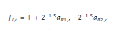
where R 1i and R 2i are respectively the first and second row of the Hadamard matrix assigned to the i -th HU, and a R l i, r and a R 2i,r are respectively the matrix elements (either 1 or −1) from the Hadamard matrix in rows R 1 i and R 2 i and column r . Note that the formula for ƒ i,r yields replicate factors that can take one of three approximate values: 1.7, 1.0, or 0.3. That is;
The expectation is that 50 percent of replicate factors will be 1, and the other 50 percent will be evenly split between 1.7 and 0.3 (Gunlicks, 1996). The following example demonstrates the computation of replicate factors for a sample of size five, using a Hadamard matrix of order four:
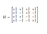
Table 12.1 presents an example of a two-row assignment developed from this matrix, and the values
of replicate factors for each sample unit.
Table 12.1 Example of Two-Row Assignment, Hadamard Matrix Elements, and Replicate Factors
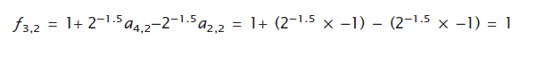
Note that row 1 is not used. For the third case ( i = 3), rows four and two of the Hadamard matrix are to calculate the replicate factors. For the second replicate ( r = 2), the replicate factor is computed using the values in the second column of rows four (−1) and two (−1) as follows:
Next, a pair of rows in the Hadamard matrix is assigned to each record (HU or group quarters (GQ) person). An algorithm is used to assign two rows of an 80×80 Hadamard matrix to each HU. The ACS uses a repeating sequence of 780 pairs of rows in the Hadamard matrix assigned to each record, in short order (Navarro, 2001a). The assignment of Hadamard matrix rows repeats every 780 records until all records receive a pair of rows from the Hadamard matrix. The first row of the matrix, in which every cell is always equal to one, is not used.
The replicate factor for each record then is determined from these two rows of the 80×80 Hadamard matrix. For record i ( i = 1, …, n , where n is sample size) and replicate r ( r = 1, …, 80), the replicate factor is computed as:
where R 1i and R 2i are respectively the first and second row of the Hadamard matrix assigned to the i -th HU, and a R l i, r and a R 2i,r are respectively the matrix elements (either 1 or −1) from the Hadamard matrix in rows R 1 i and R 2 i and column r . Note that the formula for ƒ i,r yields replicate factors that can take one of three approximate values: 1.7, 1.0, or 0.3. That is;
- If a R 1 i,r = +1 and a R 2 i,r = +1, the replicate factor is 1.
- If a R 1 i,r = −1 and a R 2 i,r = −1, the replicate factor is 1.
- If a R 1 i,r = +1 and a R 2 i,r = −1, the replicate factor is approximately 1.7.
- If a R 1 i,r = −1 and a R 2 i,r = +1, the replicate factor is approximately 0.3.
The expectation is that 50 percent of replicate factors will be 1, and the other 50 percent will be evenly split between 1.7 and 0.3 (Gunlicks, 1996). The following example demonstrates the computation of replicate factors for a sample of size five, using a Hadamard matrix of order four:
Table 12.1 presents an example of a two-row assignment developed from this matrix, and the values
of replicate factors for each sample unit.
Table 12.1 Example of Two-Row Assignment, Hadamard Matrix Elements, and Replicate Factors
| Case # (i) | Row assignment | Hadamard matrix element | Approximate replicate factor | |||||||||||
| R1i | R2i | Replicate 1 | Replicate 2 | Replicate 3 | Replicate 4 | fi,1 | fi,2 | fi,3 | fi,4 | |||||
| aR1i,1 | aR2i,1 | aR1i,2 | aR2i,2 | aR1i,3 | aR2i,3 | aR1i,4 | aR2i,4 | |||||||
| 1 | 2 | 3 | +1 | +1 | -1 | +1 | +1 | -1 | -1 | -1 | 1 | 0.3 | 1.7 | 1 |
| 2 | 3 | 4 | +1 | +1 | +1 | -1 | -1 | -1 | -1 | +1 | 1 | 1.7 | 1 | 0.3 |
| 3 | 4 | 2 | +1 | +1 | -1 | -1 | -1 | +1 | +1 | -1 | 1 | 1 | 0.3 | 1.7 |
| 4 | 2 | 3 | +1 | +1 | -1 | +1 | +1 | -1 | -1 | -1 | 1 | 0.3 | 1.7 | 1 |
| 5 | 3 | 4 | +1 | +1 | +1 | -1 | -1 | -1 | -1 | +1 | 1 | 1.7 | 1 | 0.3 |
Note that row 1 is not used. For the third case ( i = 3), rows four and two of the Hadamard matrix are to calculate the replicate factors. For the second replicate ( r = 2), the replicate factor is computed using the values in the second column of rows four (−1) and two (−1) as follows:
Replicate weights are produced in a way similar to that used to produce full sample final weights. All of the weighting adjustment processes performed on the full sample final survey weights (such as applying noninterview adjustments and population controls) also are carried out for each replicate weight. However, collapsing patterns are retained from the full sample weighting and are not determined again for each set of replicate weights.
Before applying the weighting steps explained in Chapter 11, the set of replicate sampling weights is computed. With the replicate factor assigned, the replicate sampling weight for replicate r is computed by multiplying the full sample weight after computer-assisted personal interviewing (CAPI) subsampling factor ( WSSF - see Chapter 11 for the computation of this weight) by the replicate factor f i,r ; that is, RWSSF i,r = WSST i x f i,r, where RWSSF i,r is the replicate weight after CAPI subsampling factor for the i -th HU and the r -th replicate ( r = 1, ..., 80).
One can elaborate on the previous example of the replicate construction using five cases and four replicates: Suppose the full sample WSSF values are given under the second column of the following table (Table 12.2). Then, the replicate weight after CAPI subsampling factor ( RWSSF ) values are given in columns 7-10.
Table 12.2 Example of Computation of Replicate Weight After CAPI Subsampling Factor ( RWSSF )
The rest of the weighting process (Chapter 11) then is applied to each replicate weight RWSSF i,r (starting from the adjustment for variation in monthly response ( VMS ) and proceeding to the population control adjustment or raking). Basically, the weighting adjustment process is repeated independently 80 times and the RWSSF i,r is used in place of WSSF i (as in Chapter 11). By the end of this process, 80 final replicate weights for each HU and person record are produced.
Before applying the weighting steps explained in Chapter 11, the set of replicate sampling weights is computed. With the replicate factor assigned, the replicate sampling weight for replicate r is computed by multiplying the full sample weight after computer-assisted personal interviewing (CAPI) subsampling factor ( WSSF - see Chapter 11 for the computation of this weight) by the replicate factor f i,r ; that is, RWSSF i,r = WSST i x f i,r, where RWSSF i,r is the replicate weight after CAPI subsampling factor for the i -th HU and the r -th replicate ( r = 1, ..., 80).
One can elaborate on the previous example of the replicate construction using five cases and four replicates: Suppose the full sample WSSF values are given under the second column of the following table (Table 12.2). Then, the replicate weight after CAPI subsampling factor ( RWSSF ) values are given in columns 7-10.
Table 12.2 Example of Computation of Replicate Weight After CAPI Subsampling Factor ( RWSSF )
| Case # | WSSFi | Approximate replicate factor | Replicate weight after CAPI subsampling factor | ||||||
| fi,1 | fi,2 | fi,3 | fi,4 | RWSSFi,1 | RWSSFi,2 | RWSSFi,3 | RWSSFi,4 | ||
| 1 | 100 | 1 | 0.3 | 1.7 | 1 | 100 | 29 | 171 | 100 |
| 2 | 120 | 1 | 1.7 | 1 | 0.3 | 120 | 205 | 120 | 35 |
| 3 | 80 | 1 | 1 | 0.3 | 1.7 | 80 | 80 | 23 | 137 |
| 4 | 120 | 1 | 0.3 | 1.7 | 1 | 120 | 35 | 205 | 120 |
| 5 | 110 | 1 | 1.7 | 1 | 0.3 | 110 | 188 | 110 | 32 |
The rest of the weighting process (Chapter 11) then is applied to each replicate weight RWSSF i,r (starting from the adjustment for variation in monthly response ( VMS ) and proceeding to the population control adjustment or raking). Basically, the weighting adjustment process is repeated independently 80 times and the RWSSF i,r is used in place of WSSF i (as in Chapter 11). By the end of this process, 80 final replicate weights for each HU and person record are produced.
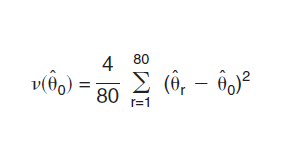
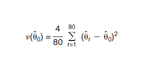
Given the replicate weights, the computation of variance for any ACS estimate is straightforward. Suppose that è is an ACS estimate of any type of statistic, such as mean, total, or proportion. Let Θ0 denote the estimate computed based on the full sample weight, and Θ1, Θ2,... Θ80, denote the estimates computed based on the replicate weights. The variance of Θ0 v( Θ0) is estimated as the sum of squared differences between each replicate estimate Θ r ( r = 1, ..., 80) and the full sample estimate Θ0. The formula is as follows:1
This equation holds for count estimates as well as any other types of estimates, including percents, ratios, and medians.
There are certain cases, however, where this formula does not apply. The first and most important cases are estimates that are "controlled" to population totals and have their standard errors set to zero. These are estimates that are forced to equal intercensal estimates during the weighting process raking step-for example, total population and collapsed age, sex, and Hispanic origin estimates for weighting areas. Although race is included in the raking procedure, race group estimates are not controlled; the categories used in the weighting process (see Chapter 11) do not match the published tabulation groups because of multiple race responses and the "Some Other Race" category. Information on the final collapsing of the person post-stratification cells is passed from the weighting to the variance estimation process in order to identify estimates that are controlled. This is done independently for all weighting areas and then is applied to the geographic areas used for tabulation. Standard errors for those estimates are set to zero, and published margins of error are set to "*****" (with an appropriate accompanying footnote).
Another special case deals with zero-estimated counts of people, households, or HUs. A direct application of the replicate variance formula leads to a zero standard error for a zero-estimated count. However, there may be people, households, or HUs with that characteristic in that area that were not selected to be in the ACS sample, but a different sample might have selected them, so a zero standard error is not appropriate. For these cases, the following model-based estimation of standard error was implemented.
For ACS data in a census year, the ACS zero-estimated counts (for characteristics included in the 100 percent census ("short form") count) can be checked against the corresponding census estimates. At least 90 percent of the census counts for the ACS zero-estimated counts should be within a 90 percent confidence interval based on our modeled standard error.2 Let the variance of the estimate be modeled as some multiple ( K ) of the average final weight (for a state or the nation). That is:
v(0) = K x (average weight)
Then, set the 90 percent upper bound for the zero estimate equal to the census count:
Solving for K yields:
K was computed for all ACS zero-estimated counts from 2000, which matched Census 2000 100 percent counts, and then the 90th percentile of those K s was determined. Based on the Census 2000 data, we use a value for K of 400 (Navarro, 2001b). As this modeling method requires census counts, the 400 value can next be updated using the 2010 Census and 2010 ACS data.
For publication, the standard error ( SE ) of the zero count estimate is computed as:
The average weights (the maximum of the average housing unit and average person final weights) are calculated at the state and national level for each ACS single-year or multiyear data release. Estimates for geographic areas within a state use that states average weight, and estimates for geographic areas that cross state boundaries use the national average weight.
Finally, a similar method is used to produce an approximate standard error for both ACS zero and 100 percent estimates. We do not produce approximate standard errors for other zero estimates, such as ratios or medians.
Footnote:
1A general replication-based variance formula can be expressed as where c r is the multiplier related to the r -th replicate determined by the replication method. For the SDR method, the value of c r is 4 / R , where R is the number of replicates (see Fay and Train, 1995).
2This modeling was done only once, in 2001, prior to the publication of the 2000 ACS data.
This equation holds for count estimates as well as any other types of estimates, including percents, ratios, and medians.
There are certain cases, however, where this formula does not apply. The first and most important cases are estimates that are "controlled" to population totals and have their standard errors set to zero. These are estimates that are forced to equal intercensal estimates during the weighting process raking step-for example, total population and collapsed age, sex, and Hispanic origin estimates for weighting areas. Although race is included in the raking procedure, race group estimates are not controlled; the categories used in the weighting process (see Chapter 11) do not match the published tabulation groups because of multiple race responses and the "Some Other Race" category. Information on the final collapsing of the person post-stratification cells is passed from the weighting to the variance estimation process in order to identify estimates that are controlled. This is done independently for all weighting areas and then is applied to the geographic areas used for tabulation. Standard errors for those estimates are set to zero, and published margins of error are set to "*****" (with an appropriate accompanying footnote).
Another special case deals with zero-estimated counts of people, households, or HUs. A direct application of the replicate variance formula leads to a zero standard error for a zero-estimated count. However, there may be people, households, or HUs with that characteristic in that area that were not selected to be in the ACS sample, but a different sample might have selected them, so a zero standard error is not appropriate. For these cases, the following model-based estimation of standard error was implemented.
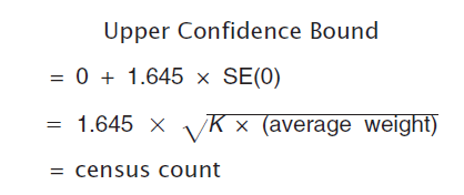
For ACS data in a census year, the ACS zero-estimated counts (for characteristics included in the 100 percent census ("short form") count) can be checked against the corresponding census estimates. At least 90 percent of the census counts for the ACS zero-estimated counts should be within a 90 percent confidence interval based on our modeled standard error.2 Let the variance of the estimate be modeled as some multiple ( K ) of the average final weight (for a state or the nation). That is:
v(0) = K x (average weight)
Then, set the 90 percent upper bound for the zero estimate equal to the census count:
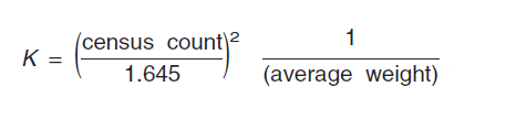
Solving for K yields:
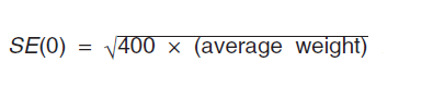
K was computed for all ACS zero-estimated counts from 2000, which matched Census 2000 100 percent counts, and then the 90th percentile of those K s was determined. Based on the Census 2000 data, we use a value for K of 400 (Navarro, 2001b). As this modeling method requires census counts, the 400 value can next be updated using the 2010 Census and 2010 ACS data.
For publication, the standard error ( SE ) of the zero count estimate is computed as:
The average weights (the maximum of the average housing unit and average person final weights) are calculated at the state and national level for each ACS single-year or multiyear data release. Estimates for geographic areas within a state use that states average weight, and estimates for geographic areas that cross state boundaries use the national average weight.
Finally, a similar method is used to produce an approximate standard error for both ACS zero and 100 percent estimates. We do not produce approximate standard errors for other zero estimates, such as ratios or medians.
Footnote:
1A general replication-based variance formula can be expressed as
where c r is the multiplier related to the r -th replicate determined by the replication method. For the SDR method, the value of c r is 4 / R , where R is the number of replicates (see Fay and Train, 1995). 2This modeling was done only once, in 2001, prior to the publication of the 2000 ACS data.
Once the standard errors have been computed, margins of error and confidence bounds are produced for each estimate. These are the measures of overall sampling error presented along with each published ACS estimate. All published ACS margins of error and the lower and upper bounds of confidence intervals presented in the ACS data products are based on a 90 percent confidence level, which is the Census Bureau's standard (U.S. Census Bureau, 2008a).
A margin of error contains two components: the standard error of the estimate, and a multiplication factor based on a chosen confidence level. For the 90 percent confidence level, the value of the multiplication factor used by the ACS is 1.645. The margin of error of an estimate è can be computed as:
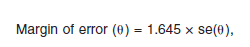
where se( Θ) is the standard error of the estimate Θ. Given this margin of error, the 90 percent confidence interval can be computed as:
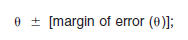
that is, the lower bound of the confidence interval is [ Θ - margin of error ( Θ) ], and the upper bound of the confidence interval is [ Θ + margin of error ( Θ) ]. Roughly speaking, this interval is a range that will contain the true value of the estimated characteristic, with a known probability.
Users are cautioned to consider "logical" boundaries when creating confidence bounds from the margins of error. For example, a small population estimate may have a calculated lower bound less than zero. A negative number of people does not make sense, so the lower bound should be set to zero instead. Likewise, bounds for percents should not go below zero percent or above 100 percent. For other characteristics, like income, negative values may be legitimate.
Given the confidence bounds, a margin of error can be computed as the difference between an estimate and its upper or lower confidence bounds:
Margin of Error = max (upper bound - estimate, estimate - lower bound)
Using the margin of error (as published or calculated from the bounds), the standard error is obtained as follows:
Standard Error = Margin of Error / 1.645
For ranking tables and comparison profiles, the ACS provides an indicator as to whether two estimates are statistically significantly different at the 90 percent confidence level. That determination is made by initially calculating:
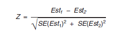
If Z < -1.645 or Z > 1.645, the difference between the estimates is significant at the 90 percent level. Determinations of statistical significance are made using unrounded values of the standard errors, so users may not be able to achieve the same result using the standard errors derived from the rounded estimates and margins of error as published. Only pairwise tests are used to determine significance in the ranking tables; no multiple comparison methods are used.
A margin of error contains two components: the standard error of the estimate, and a multiplication factor based on a chosen confidence level. For the 90 percent confidence level, the value of the multiplication factor used by the ACS is 1.645. The margin of error of an estimate è can be computed as:
where se( Θ) is the standard error of the estimate Θ. Given this margin of error, the 90 percent confidence interval can be computed as:
that is, the lower bound of the confidence interval is [ Θ - margin of error ( Θ) ], and the upper bound of the confidence interval is [ Θ + margin of error ( Θ) ]. Roughly speaking, this interval is a range that will contain the true value of the estimated characteristic, with a known probability.
Users are cautioned to consider "logical" boundaries when creating confidence bounds from the margins of error. For example, a small population estimate may have a calculated lower bound less than zero. A negative number of people does not make sense, so the lower bound should be set to zero instead. Likewise, bounds for percents should not go below zero percent or above 100 percent. For other characteristics, like income, negative values may be legitimate.
Given the confidence bounds, a margin of error can be computed as the difference between an estimate and its upper or lower confidence bounds:
Margin of Error = max (upper bound - estimate, estimate - lower bound)
Using the margin of error (as published or calculated from the bounds), the standard error is obtained as follows:
Standard Error = Margin of Error / 1.645
For ranking tables and comparison profiles, the ACS provides an indicator as to whether two estimates are statistically significantly different at the 90 percent confidence level. That determination is made by initially calculating:
If Z < -1.645 or Z > 1.645, the difference between the estimates is significant at the 90 percent level. Determinations of statistical significance are made using unrounded values of the standard errors, so users may not be able to achieve the same result using the standard errors derived from the rounded estimates and margins of error as published. Only pairwise tests are used to determine significance in the ranking tables; no multiple comparison methods are used.
The Census Bureau cannot possibly predict all combinations of estimates and geography that may be of interest to data users. Data users can download PUMS files and tabulate the data to create estimates of their own choosing. The ACS PUMS contains a subset of the full ACS sample. Thus, estimates from the ACS PUMS file can be different from the published ACS estimates that are based on the full ACS sample.
Users of the ACS PUMS files can compute the estimated variances of their statistics using one of two options: (1) the replication method using replicate weights released with the PUMS data, and (2) the design factor method described below.
For the replicate method, direct variance estimates based on the SDR formula as described in Section B above can be implemented. Users can simply tabulate 80 replicate estimates in addition to their desired estimate by using the provided 80 replicate weights, and apply the variance formula:
Similar to methods used to calculate standard errors for PUMS data from Census 2000, the ACS PUMS provides tables of design factors for various topics such as age for persons or tenure for HUs. The 2007 ACS PUMS design factors are published at national and state levels (U.S. Census Bureau, 2008b), and were calculated using 2005 ACS data. PUMS design factors will be updated periodically, but not on an annual basis. The design factor approach was developed based on a model that uses a standard error from a simple random sample as the base, and then inflates it to account for an increase in the variance caused by the complex sample design. Standard errors for almost all counts and proportions of persons, households, and HUs are approximated using design factors. For single-year ACS PUMS files beginning with 2005, use:
for a total, and
for a percent,
where
Y = the estimate of total or a count.
p = the estimate of a percent.
DF = the appropriate design factor based on the topic of the estimate.
N = the total for the geographic area of interest (if the estimate is of HUs, the number of HUs is used; if the estimate is of families or households, the number of households is used; otherwise the number of persons is used as N ).
B = the base (denominator) of a percent.
The factor 99 in the formula is the value of the finite population correction factor for the PUMS, which is computed as (100 - f ) / f , where f (given as a percent) is the sampling rate for the PUMS data. Since the PUMS is approximately a 1 percent sample of HUs, (100 - f ) / f = (100 - 1) /1 = 99.
For 3-year PUMS files beginning with 2005−2007, the 3 years worth of data represent approximately a 3 percent sample of HUs. Hence, the finite population correction factor for 3-year PUMS is (100 - f ) / f = (100 - 3) / 3 = 97 / 3. To calculate standard errors from 3-year PUMS data, substitute 97 / 3 for 99 in the above formulas.
The design factor ( DF ) is defined as the ratio of the standard error of an estimated parameter (computed under the replication method described in Section B) to the standard error based on a simple random sample of the same size. The DF reflects the effect of the actual sample design and estimation procedures used for the ACS. The DF for each topic was computed by modeling the relationship between the standard error under the replication method ( RSE ) with the standard error based on a simple random sample ( SRSSE ); that is, RSE = DF x SRSSE , where the SRSSE is computed as follows:
The value 39 in the formula above is the finite population correction factor based on an approximate sampling fraction of 2.5 percent in the ACS; that is, 100 - 2.5) / 2.5 = 97.5 / 2.5 = 39.
The value of DF is obtained by fitting this (no intercept) regression model RSE = DF x SRSSE using standard errors ( RSE , SRSSE ) for various published table estimates at the national and state levels. The values of DF s by topic can be obtained from the PUMS Accuracy of the Data (2007) (U.S. Census Bureau, 2008b). The documentation also provides examples on how to use the design factor GVFs to compute standard errors for the estimates of totals, means, medians, proportions or percentages, ratios, sums, and differences.
The topics for the 2007 PUMS design factors are, for the most part, the same ones that were available for the Census 2000 PUMS. We recommend to users that, in using the design factor approach, if the estimate is a combination of two or more characteristics, the largest DF for this combination of characteristics is used. The only exceptions to this are items crossed with race or Hispanic origin; for these items, the largest DF is used, excluding race or Hispanic origin DF s.
Users of the ACS PUMS files can compute the estimated variances of their statistics using one of two options: (1) the replication method using replicate weights released with the PUMS data, and (2) the design factor method described below.
For the replicate method, direct variance estimates based on the SDR formula as described in Section B above can be implemented. Users can simply tabulate 80 replicate estimates in addition to their desired estimate by using the provided 80 replicate weights, and apply the variance formula:
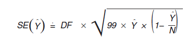
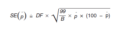
Similar to methods used to calculate standard errors for PUMS data from Census 2000, the ACS PUMS provides tables of design factors for various topics such as age for persons or tenure for HUs. The 2007 ACS PUMS design factors are published at national and state levels (U.S. Census Bureau, 2008b), and were calculated using 2005 ACS data. PUMS design factors will be updated periodically, but not on an annual basis. The design factor approach was developed based on a model that uses a standard error from a simple random sample as the base, and then inflates it to account for an increase in the variance caused by the complex sample design. Standard errors for almost all counts and proportions of persons, households, and HUs are approximated using design factors. For single-year ACS PUMS files beginning with 2005, use:
for a total, and
for a percent,
where
Y = the estimate of total or a count.
p = the estimate of a percent.
DF = the appropriate design factor based on the topic of the estimate.
N = the total for the geographic area of interest (if the estimate is of HUs, the number of HUs is used; if the estimate is of families or households, the number of households is used; otherwise the number of persons is used as N ).
B = the base (denominator) of a percent.
The factor 99 in the formula is the value of the finite population correction factor for the PUMS, which is computed as (100 - f ) / f , where f (given as a percent) is the sampling rate for the PUMS data. Since the PUMS is approximately a 1 percent sample of HUs, (100 - f ) / f = (100 - 1) /1 = 99.
For 3-year PUMS files beginning with 2005−2007, the 3 years worth of data represent approximately a 3 percent sample of HUs. Hence, the finite population correction factor for 3-year PUMS is (100 - f ) / f = (100 - 3) / 3 = 97 / 3. To calculate standard errors from 3-year PUMS data, substitute 97 / 3 for 99 in the above formulas.
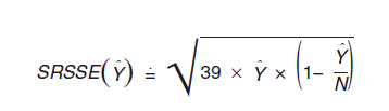
The design factor ( DF ) is defined as the ratio of the standard error of an estimated parameter (computed under the replication method described in Section B) to the standard error based on a simple random sample of the same size. The DF reflects the effect of the actual sample design and estimation procedures used for the ACS. The DF for each topic was computed by modeling the relationship between the standard error under the replication method ( RSE ) with the standard error based on a simple random sample ( SRSSE ); that is, RSE = DF x SRSSE , where the SRSSE is computed as follows:
The value 39 in the formula above is the finite population correction factor based on an approximate sampling fraction of 2.5 percent in the ACS; that is, 100 - 2.5) / 2.5 = 97.5 / 2.5 = 39.
The value of DF is obtained by fitting this (no intercept) regression model RSE = DF x SRSSE using standard errors ( RSE , SRSSE ) for various published table estimates at the national and state levels. The values of DF s by topic can be obtained from the PUMS Accuracy of the Data (2007) (U.S. Census Bureau, 2008b). The documentation also provides examples on how to use the design factor GVFs to compute standard errors for the estimates of totals, means, medians, proportions or percentages, ratios, sums, and differences.
The topics for the 2007 PUMS design factors are, for the most part, the same ones that were available for the Census 2000 PUMS. We recommend to users that, in using the design factor approach, if the estimate is a combination of two or more characteristics, the largest DF for this combination of characteristics is used. The only exceptions to this are items crossed with race or Hispanic origin; for these items, the largest DF is used, excluding race or Hispanic origin DF s.
Fay, R., and G. Train. (1995). "Aspects of Survey and Model-Based Postcensal Estimation of Income and Poverty Characteristics for States and Counties." Proceedings of the Section on Government Statistics . Alexandria, VA: American Statistical Association, pp. 154−159, .
Gbur, P., and L. Fairchild. (2002). "Overview of the U.S. Census 2000 Long Form Direct Variance Estimation." Proceedings of the Section on Survey Research Methods . Alexandria, VA: American Statistical Association, pp. 1139−1144.
Gunlicks, C. (1996). "1990 Replicate Variance System (VAR90-20)." Internal U.S. Census Bureau Memorandum for Documentation, June 4, 1996.
Judkins, D. R. (1990). "Fays Method for Variance Estimation." Journal of Official Statistics, Vol. 6, No. 3, 1990, pp. 223−239.
Navarro, A. (2001a). "2000 American Community Survey (ACS) Comparison County Replicate Factors (ACS-V-01)." Internal U.S. Census Bureau Memorandum to C. Alexander, Washington, DC, May 23, 2001.
Navarro, A. (2001b). "Estimating Standard Errors of Zero Estimates." Internal U.S. Census Bureau Draft Memorandum to C. Alexander, Washington, DC, November 6, 2001.
U.S. Census Bureau (2002). "Current Population Survey: Technical Paper 63RV-Design and Methodology." Washington, DC, 2002,.
U.S. Census Bureau (2008a). "Census Bureau Standard: Dissemination of Census and Survey Data Products." Washington, DC, 2008,.
U.S. Census Bureau (2008b). "PUMS Accuracy of the Data (2007)." Washington, DC, 2008,. Wolter, K. M. (1984). "An Investigation of Some Estimators of Variance for Systematic Sampling." Journal of the American Statistical Association , Vol. 79, 1984, pp. 781−790.
Gbur, P., and L. Fairchild. (2002). "Overview of the U.S. Census 2000 Long Form Direct Variance Estimation." Proceedings of the Section on Survey Research Methods . Alexandria, VA: American Statistical Association, pp. 1139−1144.
Gunlicks, C. (1996). "1990 Replicate Variance System (VAR90-20)." Internal U.S. Census Bureau Memorandum for Documentation, June 4, 1996.
Judkins, D. R. (1990). "Fays Method for Variance Estimation." Journal of Official Statistics, Vol. 6, No. 3, 1990, pp. 223−239.
Navarro, A. (2001a). "2000 American Community Survey (ACS) Comparison County Replicate Factors (ACS-V-01)." Internal U.S. Census Bureau Memorandum to C. Alexander, Washington, DC, May 23, 2001.
Navarro, A. (2001b). "Estimating Standard Errors of Zero Estimates." Internal U.S. Census Bureau Draft Memorandum to C. Alexander, Washington, DC, November 6, 2001.
U.S. Census Bureau (2002). "Current Population Survey: Technical Paper 63RV-Design and Methodology." Washington, DC, 2002,
U.S. Census Bureau (2008a). "Census Bureau Standard: Dissemination of Census and Survey Data Products." Washington, DC, 2008,
U.S. Census Bureau (2008b). "PUMS Accuracy of the Data (2007)." Washington, DC, 2008,

