


| Documentation: | ACS 2009 (1-Year Estimates) |
you are here:
choose a survey
survey
document
chapter
Publisher: U.S. Census Bureau
Survey: ACS 2009 (1-Year Estimates)
| Document: | Design and Methodology: American Community Survey |
| citation: | Social Explorer; U.S. Census Bureau; Design and Methodology, American Community Survey. U.S. Government Printing Office, Washington, DC, 2009. |
Chapter Contents
Beginning in 2010, the U.S. Census Bureau plans to release three sets of American Community Survey (ACS) estimates annually for specified geographic areas, using data collected over three different periods. In general, the Census Bureau will produce and publish estimates for the same set of statistical, legal, and administrative entities as the previously published Census long form: the nation, states, American Indian and Alaska Native (AIAN) areas, counties ( municipios in Puerto Rico), minor civil divisions (MCDs), incorporated places, and census tracts, among others (see Chapter 8.B). The Census Bureau will publish up to three sets of estimates for a geographic area depending on its total population.
The basic estimation approach is a ratio estimation procedure that results in the assignment of two sets of weights: a weight to each sample person record, both household and group quarters (GQ) persons, and a weight to each sample housing unit (HU) record. Ratio estimation is a method that takes advantage of auxiliary information (in this case, population estimates by sex, age, race, and Hispanic origin, and estimates of total HUs) to increase the precision of the estimates as well as correct for differential coverage by geography and demographic detail. This method also produces ACS estimates consistent with the population estimates from the Population Estimates Program (PEP) of the Census Bureau by these characteristics and the estimates of total HUs for each county in the United States.
For any given tabulation area, a characteristic total is estimated by summing the weights assigned to the people, households, families, or HUs possessing the characteristic. Estimates of population characteristics are based on the person weight. Estimates of family, household, and HU characteristics are based on the HU weight. As with most household surveys, weights are used to bring the characteristics of the sample more into agreement with those of the full population by compensating for differences in sampling rates across areas, differences between the full sample and the interviewed sample, and differences between the sample and independent estimates of basic demographic characteristics (Alexander et al., 1997).
Section B describes the 2007 single-year weighting methodology for calculating person weights for the GQ sample records. This weighting for GQ persons is done independently of the weighting for HUs. Sections C, D, E, and F describe the 2007 single-year weighting methodology for calculating HU weights and person weights for the household sample records. The weighting for household persons makes use of the GQ person weights so that the household and GQ person weights can be combined to produce estimates of the total population. While the methodology for the multiyear weighting is largely the same as the single-year weighting methodology, Section G outlines where the 2005−2007 3-year weighting methodology differs from the 2007 single-year methodology.
- The Census Bureau plans to publish multiyear estimates based on 5 calendar years of sample data for all statistical, legal, and administrative entities, including census tracts, block groups, and small incorporated places, such as cities and towns. These 5-year estimates are based on data collected during the 60 months of the 5 most recent collection years.
- For geographic entities with populations of at least 20,000, the Census Bureau will also publish 3-year estimates based on data collected during the 36 months of the 3 most recent collection years.
- For geographic entities with populations of at least 65,000, the Census Bureau will also publish single-year estimates based on data collected during the 12 months of the most recent calendar year.
The basic estimation approach is a ratio estimation procedure that results in the assignment of two sets of weights: a weight to each sample person record, both household and group quarters (GQ) persons, and a weight to each sample housing unit (HU) record. Ratio estimation is a method that takes advantage of auxiliary information (in this case, population estimates by sex, age, race, and Hispanic origin, and estimates of total HUs) to increase the precision of the estimates as well as correct for differential coverage by geography and demographic detail. This method also produces ACS estimates consistent with the population estimates from the Population Estimates Program (PEP) of the Census Bureau by these characteristics and the estimates of total HUs for each county in the United States.
For any given tabulation area, a characteristic total is estimated by summing the weights assigned to the people, households, families, or HUs possessing the characteristic. Estimates of population characteristics are based on the person weight. Estimates of family, household, and HU characteristics are based on the HU weight. As with most household surveys, weights are used to bring the characteristics of the sample more into agreement with those of the full population by compensating for differences in sampling rates across areas, differences between the full sample and the interviewed sample, and differences between the sample and independent estimates of basic demographic characteristics (Alexander et al., 1997).
Section B describes the 2007 single-year weighting methodology for calculating person weights for the GQ sample records. This weighting for GQ persons is done independently of the weighting for HUs. Sections C, D, E, and F describe the 2007 single-year weighting methodology for calculating HU weights and person weights for the household sample records. The weighting for household persons makes use of the GQ person weights so that the household and GQ person weights can be combined to produce estimates of the total population. While the methodology for the multiyear weighting is largely the same as the single-year weighting methodology, Section G outlines where the 2005−2007 3-year weighting methodology differs from the 2007 single-year methodology.
Since the 2006 data collection year, estimates from the ACS have included data from both people living in both HUs and GQs. The weighting of GQ persons is performed in three major steps. The first step calculates the sampling base weights, which includes adjustments for subsampling that occurs at the time of interview. The second step adjusts the interviewed person records for nonresponse. The third step adjusts the person weights so that the weighted estimates conform to estimates from the PEP at the state by major GQ type group level. The basic weighting area used for the GQ weighting is the state.
The sampling of GQ persons has two phases-the initial sampling of hits and the subsampling of GQ persons associated with those hits (see Chapter 4 for more details). The initial sampling of GQ persons has a uniform sampling rate of 2.5 percent. Thus, the initial base weight ( BW ) for all GQ persons is equal to the inverse of the sampling rate, 40. This initial weight reflects the sampling probability of the sample hit and the within-GQ sampling probability of the persons if the population of the GQ is equal to the expected value given on the frame. If the observed population is different from the expected value on the frame, then the within-GQ sampling rate will be adjusted to select the same number of sample persons and the weights need to be adjusted accordingly. This adjusted base weight is called the preliminary final base weight ( PFBW ).
The adjustment of the initial base weight ( BW ) for the subsampling that occurs at the time of interview depends on whether the GQ remains in the size stratum that it was initially assigned at the time of sampling based on the new observed population.
GQs in the small size stratum (those whose expected population are 15 or fewer) that remain in the small size stratum based on their observed population will keep their original base weight of 40 since a take-all procedure is used as long as the observed population is 15 or fewer. However, if the small GQ has an observed population of 16 or more, a subsampling procedure is performed to select 10 GQ residents to interview. The base weight in this case is adjusted by the "take every x resident" necessary to select the 10 residents.
GQs in the large size stratum (those whose expected population are 16 or more) will have their base weight adjusted in all situations where the observed population differs from the expected population of the GQ. If the observed size of the large GQ is 10 or more, the base weight is adjusted by the ratio of the observed population to the expected population. If the observed size is fewer than 10 persons, then the base weight is adjusted by the fraction of 10 over the expected size. These adjustments to the initial base weight are summarized in Table 11-1.
Table 11.1 Calculation of the Preliminary Final Base Weight ( PFBW )
The final step in calculating the sampling weights is a weight-trimming procedure. This procedure caps all preliminary final base weights at 350 and then spreads the excess weight via a ratio adjustment to other GQ person interviews within the same state and major GQ type group. The type groups are defined in Table 11.2. The resulting weights after trimming are then defined as the final base weights ( FBW ) that include all sampling probabilities with the trimming applied.
Table 11.2 Major GQ Type Groups
The adjustment of the initial base weight ( BW ) for the subsampling that occurs at the time of interview depends on whether the GQ remains in the size stratum that it was initially assigned at the time of sampling based on the new observed population.
GQs in the small size stratum (those whose expected population are 15 or fewer) that remain in the small size stratum based on their observed population will keep their original base weight of 40 since a take-all procedure is used as long as the observed population is 15 or fewer. However, if the small GQ has an observed population of 16 or more, a subsampling procedure is performed to select 10 GQ residents to interview. The base weight in this case is adjusted by the "take every x resident" necessary to select the 10 residents.
GQs in the large size stratum (those whose expected population are 16 or more) will have their base weight adjusted in all situations where the observed population differs from the expected population of the GQ. If the observed size of the large GQ is 10 or more, the base weight is adjusted by the ratio of the observed population to the expected population. If the observed size is fewer than 10 persons, then the base weight is adjusted by the fraction of 10 over the expected size. These adjustments to the initial base weight are summarized in Table 11-1.
Table 11.1 Calculation of the Preliminary Final Base Weight ( PFBW )
| Size stratum at time of sampling | Observed population | ||
|---|---|---|---|
| Less than 10 persons | 11 to 15 persons | 16 or more persons | |
| Small stratum | BW | BW | BW * (Observed population) /10 |
| Large stratum | BW * 10 / (Expected population) | BW * (Observed population) / (Expected population) | BW * (Observed population) / (Expected population) |
The final step in calculating the sampling weights is a weight-trimming procedure. This procedure caps all preliminary final base weights at 350 and then spreads the excess weight via a ratio adjustment to other GQ person interviews within the same state and major GQ type group. The type groups are defined in Table 11.2. The resulting weights after trimming are then defined as the final base weights ( FBW ) that include all sampling probabilities with the trimming applied.
Table 11.2 Major GQ Type Groups
| Major GQ type group | Definition | Institutional/Noninstitutional |
|---|---|---|
| 1 | Correctional institutions | Institutional |
| 2 | Juvenile detention facilities | Institutional |
| 3 | Nursing homes | Institutional |
| 4 | Other Llng-term care facilities | Institutional |
| 5 | College dormitories | Noninstitutional |
| 6 | Military facilities | Noninstitutional |
| 7 | Other noninstitutional facilities | Noninstitutional |
A noninterview adjustment factor is calculated to account for the eligible GQ residents who do not complete an interview. This occurs in a single step where the noninterview adjustment cells are defined, within state, by major GQ type group by county. If a cell contains fewer than 10 interviews and has any number of noninterviews or if the noninterview factor is greater than 2, then cells are collapsed across counties within the same major GQ type group in an attempt to preserve the state by type group weighted totals. If the new collapsed cell still fails one or both of the collapsing criteria, then it is collapsed to a subset of the type groups within the same institutional/ noninstitutional class as shown in Table 11.2. If needed, all cells with the same institutional/ noninstitutional class are collapsed together across all type groups in the class. If further collapsing is still required, then all cells within the state are collapsed together. In practice, these last two collapsings are rarely, if ever, used. The GQ Noninterview Adjustment Factor ( GQNIF ) for each eligible cell is then calculated:
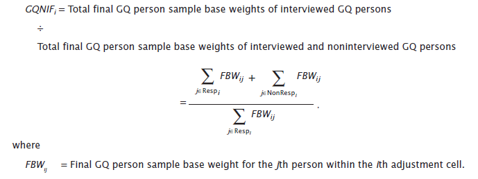
All interviewed GQ persons are adjusted by this noninterview factor. All noninterviews including those persons who were found to be out-of-scope are assigned a factor of 0.0. The computation of the weight after the noninterview adjustment factor is summarized in Table 11.3.
Table 11.3 Computation of the Weight After the GQ Noninterview Adjustment Factor ( WGQNIF )
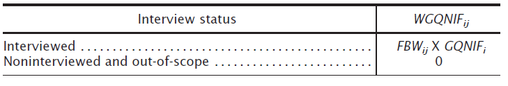
The third and last step in the GQ person weighting process is to apply the GQ Person Post- Stratification Factor ( GQPPSF ). In 2004, a project was undertaken to research an adequate method for applying controls in the single-year weighting of both the household and GQ persons (see Weidman et al., 2007, for more details). The goal of that research was to determine what was the best method to achieve, as a primary goal, accurate estimates for GQ characteristics at the state
level while also achieving, as a secondary goal, reasonable estimates for the total population at the county level. The research compared four alternative options for controlling GQ persons, either separately or in combination with HU persons. The results showed that it is feasible to control the GQ data at the state level by major GQ type group and combine those results with the weighting of the household population by weighting area to produce adequate estimates of the total population for all levels of aggregation. The choice of this methodology is further supported by the nature of the PEP GQ population estimates which are updated and maintained by major GQ type group.
The post-stratification cells are defined by state by major GQ type group and all sample interview persons are placed in their appropriate cells. If a cell contains fewer than 10 GQ persons or the ratio of the PEP population estimate to the ACS estimate calculated using the WGQNIF weight is outside of the interval 1/3.5 to 3.5, then the cell is collapsed to a subset of the type groups within the same institutional/noninstitutional class as was done for the noninterview adjustment collapsing. If the new cell fails one or both criteria, then all cells within the same institutional/ noninstitutional class are collapsed together. If further collapsing is required, then all cells within the state are collapsed together. In practice, most cells pass the criterion with either no collapsing or collapsing to a subset of the type groups within the same institutional/noninstitutional class. The GQ Person Post-Stratification Factor ( GQPPSF ) for each eligible cell is then calculated:
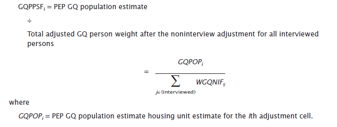
Multiplying the GQPPSF by the weighting after the GQ noninterview adjustments, WGQNIF , results in the final unrounded GQ person weight, WGQPPSF . These weights are then rounded to form the final GQ person weights.
level while also achieving, as a secondary goal, reasonable estimates for the total population at the county level. The research compared four alternative options for controlling GQ persons, either separately or in combination with HU persons. The results showed that it is feasible to control the GQ data at the state level by major GQ type group and combine those results with the weighting of the household population by weighting area to produce adequate estimates of the total population for all levels of aggregation. The choice of this methodology is further supported by the nature of the PEP GQ population estimates which are updated and maintained by major GQ type group.
The post-stratification cells are defined by state by major GQ type group and all sample interview persons are placed in their appropriate cells. If a cell contains fewer than 10 GQ persons or the ratio of the PEP population estimate to the ACS estimate calculated using the WGQNIF weight is outside of the interval 1/3.5 to 3.5, then the cell is collapsed to a subset of the type groups within the same institutional/noninstitutional class as was done for the noninterview adjustment collapsing. If the new cell fails one or both criteria, then all cells within the same institutional/ noninstitutional class are collapsed together. If further collapsing is required, then all cells within the state are collapsed together. In practice, most cells pass the criterion with either no collapsing or collapsing to a subset of the type groups within the same institutional/noninstitutional class. The GQ Person Post-Stratification Factor ( GQPPSF ) for each eligible cell is then calculated:
Multiplying the GQPPSF by the weighting after the GQ noninterview adjustments, WGQNIF , results in the final unrounded GQ person weight, WGQPPSF . These weights are then rounded to form the final GQ person weights.
Single-year weighting is implemented in three stages. In the first stage, weights are computed to account for differential selection probabilities based on the sampling rates used to select the HU sample. In the second stage, weights of responding HUs are adjusted to account for nonresponding HUs. In the third stage, weights are controlled so that the weighted estimates of HUs and persons by age, sex, race, and Hispanic origin conform to estimates from the PEP of the Census Bureau at a specific point in time. The estimation methodology is implemented by "weighting area," either a county or a group of less populous counties.
The first stage of weighting involves two steps. In the first step, each HU is assigned a basic sampling weight that accounts for the sampling probabilities in both the first and second phases of sample selection. Chapter 4 provides more details on the sampling. In the second step, these sampling weights are adjusted to reduce variability in the monthly weighted totals.
The first step is to compute the basic sampling weight for the HU based on the inverse of the probability of selection. This sampling weight is computed as a multiplication of the base weight ( BW ) and a computer-assisted personal interviewing (CAPI) subsampling factor ( SSF ). The BW for an HU is calculated as the inverse of the final overall first-phase sampling rate as given in Chapter 4, Table 4.2. HUs sent to CAPI are eligible to be subsampled (second-phase sampling) at one of the rates described in Table 4.4. Those selected for the CAPI subsample, and for which no late mail return is received in the CAPI month, are assigned a CAPI SSF equal to the inverse of their (second-phase) subsampling rate. Those not selected for the CAPI subsample receive a factor of 0.0. HUs for which a completed mail return is received, regardless if it was eligible for CAPI, or a computer-assisted telephone interviewing (CATI) interview is completed receive a CAPI SSF of 1.0. The CAPI SSF is then used to calculate a new weight for every HU, the weight after CAPI subsampling factor ( WSSF ). It is equal to the base weight times the CAPI subsampling factor. After each of the subsequent weighting steps, with one exception that will be noted, a new weight is calculated as the product of the new factor and the weight following the previous step. For additional details about the weighting steps discussed in this and the following section, see Asiala (2004).
Table 11.4 Computation of the Weight After CAPI Subsampling Factor ( WSSF )
Note: Table summarizes computation of the WSSF by the weighting step and the sample dispostion.
Table 11.4 Computation of the Weight After CAPI Subsampling Factor ( WSSF )
| Weighting step | Sample disposition | ||||
|---|---|---|---|---|---|
| Mail respondent | CATI respondendent | CAPI sampled units | CAPI nonsampled units | CAPI eligible, but then becomes mail respondent | |
| Base Weight (BW) | 1 ÷ (overall sampling rate) | 1 ÷ overall sampling rate) | 1 ÷ (overall sampling rate) | 1 ÷ (overall sampling rate) | 1 ÷ (overall sampling rate) |
| CAPI subsampling factor (SSF) | 1 | 1 | 1 ÷ (CAPI sub- sampling rate) | 0 | 1 |
| Weight after subsampling factor (WSSF)= BW × SSF | 1 ÷ (overall sampling rate) | 1 ÷ (overall sampling rate) | 1 ÷ (overall sampling rate) × 1 ÷ (CAPI sub- sampling rate) | 0 | 1 ÷ (overall sampling rate) |
Note: Table summarizes computation of the WSSF by the weighting step and the sample dispostion.
The goal of ACS estimation is to represent the characteristics of a geographic area across the specified period. For single-year estimates, this period is 12 months, and for 3- and 5-year estimates, it is 36 and 60 months, respectively. The annual sample is allocated into 12 monthly samples. The monthly sample becomes a basis for the operations of the ACS data collection, preparation, and processing, including weighting and estimation.
The data for HUs assigned to any sample month can be collected at any time during a 3-month period. For example, the households in the January sample month can have their data collected in January, February, or March. Each HU in a sample belongs to a tabulation month (the month the interview is completed). This is either the month the processing center checked in the completed mail questionnaire or the month the interview is completed by CATI or CAPI.
Because of seasonal variations in response patterns, the number of HUs in tabulation months may vary, thereby over-representing some months and under-representing other months in the single and multiyear estimates. For this reason, an even distribution of HU weights by month is desirable. To smooth out the total weight for all sample months, a variation in monthly response factor ( VMS ) is calculated for each month as:
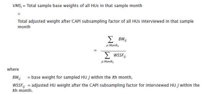
This adjustment factor is computed within each of the 2,005 ACS weighting areas (either a county or a group of less populous counties). The index for weighting area is suppressed in this and all other formulas for weighting adjustment factors.
Table 11.5 illustrates the computation of the VMS adjustment factor within a particular county. In this example, the total base weight ( BW ) for each month is 100 (as shown on line 1 of this table). The total weight ( WSSF ) across modes within each month varies from 90 to 115 (as shown on line 5). The VMS factors are then computed by month as the ratio of the total BW to the total WSSF (as shown on line 6).
Table 11.5 Example of Computation of VMS
The adjusted weights after the variation of monthly response adjustment ( WVMS ) are a product of the weights after CAPI subsampling factor ( WSSF ) and the variation of monthly response factor ( VMS ). When the VMS factor is applied, the total VMS weights ( WVMS ) across all HUs tabulated in a sample month will be equal to the total base weight of all HUs selected in that months sample. The result is that each month contributes approximately 1/12 to the total single-year estimates. In other words, the single-year estimates of ACS characteristics are a 12-month average without over- or under-representing any single month due to variation in monthly response. Analogously, each month contributes approximately 1/36 and 1/60 to the 3- and 5-year estimates, respectively.
The data for HUs assigned to any sample month can be collected at any time during a 3-month period. For example, the households in the January sample month can have their data collected in January, February, or March. Each HU in a sample belongs to a tabulation month (the month the interview is completed). This is either the month the processing center checked in the completed mail questionnaire or the month the interview is completed by CATI or CAPI.
Because of seasonal variations in response patterns, the number of HUs in tabulation months may vary, thereby over-representing some months and under-representing other months in the single and multiyear estimates. For this reason, an even distribution of HU weights by month is desirable. To smooth out the total weight for all sample months, a variation in monthly response factor ( VMS ) is calculated for each month as:
This adjustment factor is computed within each of the 2,005 ACS weighting areas (either a county or a group of less populous counties). The index for weighting area is suppressed in this and all other formulas for weighting adjustment factors.
Table 11.5 illustrates the computation of the VMS adjustment factor within a particular county. In this example, the total base weight ( BW ) for each month is 100 (as shown on line 1 of this table). The total weight ( WSSF ) across modes within each month varies from 90 to 115 (as shown on line 5). The VMS factors are then computed by month as the ratio of the total BW to the total WSSF (as shown on line 6).
Table 11.5 Example of Computation of VMS
| Line | Month | ||||
|---|---|---|---|---|---|
| March | April | May | June | July | |
| Line 1: Total base weight (BW) across released samples Total weight after CAPI subsampling (WSSF)by mode: | 100 | 100 | 100 | 100 | 100 |
| Line 2: (a) Mail | 55 (Mar sample) | 45 (Apr sample) | 40 (May sample) | 45 (Jun sample) | 50 (Jul sample) |
| Line 3: (b) CATI | 30 (Feb sample) | 25 (Mar sample) | 30 (Apr sample) | 30 (May sample) | 25 (Jun sample) |
| Line 4: (c) CAPI | 30 (Jan sample) | 25 (Feb sample) | 20 (Mar sample) | 25 (Apr sample) | 30 (May Sample) |
| Line 5: Total weight WSSF across modes (a+b+c) | 115 | 95 | 90 | 100 | 105 |
| Line 6: VMS adjustment factor | 100 ÷ 115 | 100 ÷ 95 | 100 ÷ 90 | 100 ÷ 100 | 100 ÷ 105 |
The adjusted weights after the variation of monthly response adjustment ( WVMS ) are a product of the weights after CAPI subsampling factor ( WSSF ) and the variation of monthly response factor ( VMS ). When the VMS factor is applied, the total VMS weights ( WVMS ) across all HUs tabulated in a sample month will be equal to the total base weight of all HUs selected in that months sample. The result is that each month contributes approximately 1/12 to the total single-year estimates. In other words, the single-year estimates of ACS characteristics are a 12-month average without over- or under-representing any single month due to variation in monthly response. Analogously, each month contributes approximately 1/36 and 1/60 to the 3- and 5-year estimates, respectively.
The noninterview adjustment uses three factors to account for sample HUs for which an interview is not completed. During data collection, nothing new is learned about the HU or person characteristics of noninterviewed HUs, so only characteristics known at the time of sampling can be used in adjusting for them. In other surveys and censuses, characteristics that have been shown to be related to HU response include census tract, building type (single- versus multiunit structure), and month of data collection (Weidman et al., 1995). Within counties, if a sufficient number of sample HUs were available to fill the cells of a three-way cross-classification table formed by these variables, a simultaneous adjustment for these three factors could occur. There are more than 65,000 tracts, however, so there would not be enough sample for even the two-way cross-classification of tract by month of data collection. As a result, the noninterview adjustment is carried out in two steps-one based on building type and census tract, and one based on building type and tabulation month. Once these steps are completed and the factors are applied, the sum of the weights of the interviewed HUs will equal the sum of the VMS weights of the interviewed plus noninterviewed HUs.
Note that vacant units and ineligible units such as deletes are excluded from the noninterview adjustment.1 The weight corresponding to these HUs remains unchanged during this stage of the weighting process since it is assumed that all vacant units and deletes are properly identified in the field and therefore are not eligible for the noninterview adjustment. The weighting adjustment is carried out only for the occupied, temporarily occupied (those HUs which are occupied but whose occupants do not meet the ACS residency criteria), and noninterviewed HUs. After completion of the adjustment to the weights of the interviewed HUs, the noninterviewed HUs can be dropped from subsequent weighting steps; their assigned weights will be equal to 0.
The noninterview adjustment steps are applied to all HUs interviewed by any mode-mail, CATI, or CAPI. However, nearly all noninterviewed HUs belong to the CAPI sample, so characteristics of CAPI nonrespondents may be closer to those of CAPI respondents than to mail and CATI respondents. To account for this possible mode-related noninterview bias, a mode noninterview adjustment factor is computed after the two previously mentioned noninterview adjustment steps.
Footnote:
1Deletes or out-of-scope addresses fall into three categories: (1) addresses of living quarters that have been demolished, condemned, or are uninhabitable because they are open to the elements; (2) addresses that do not exist; (3) addresses that identify commercial establishments, units being used permanently for storage, or living arrangements known as group quarters.
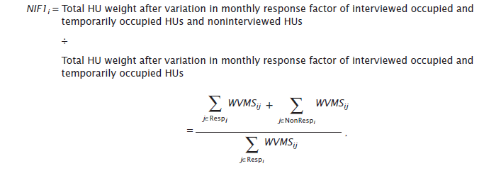
In this step, all HUs are placed into adjustment cells based on the cross-classification of building type (single- versus multiunit structures) and census tract. If a cell contains fewer than 10 interviewed HUs, it is collapsed with an adjoining tract until the collapsed cell meets the minimum size of 10.2 Cells with no noninterviews are not collapsed, regardless of size, unless they are forced to collapse with a neighboring cell that fails the size criterion. The first noninterview adjustment factor ( NIF1 ) for each eligible cell is:
Footnote:
2Data are sorted by the weighting area, building type, and tract. Within a building type, a tract that has 10 or more responses is put in its own tract. A tract that has no nonresponses and some responses (even though the total is fewer than 10) is put in its own tract. A tract that has nonresponses and fewer than 10 responses is collapsed with the next tract. If the final tract needs to be collapsed, it is collapsed with the previous tract.
where
WVMS ij = Adjusted HU weight after the variation in monthly response adjustment for the j th HU within the i th adjustment cell.
All occupied and temporarily occupied interviewed HUs are adjusted by this first noninterview factor. Vacant and deleted HUs are assigned a factor of 1.0, and noninterviews are assigned a factor of 0.0. The computation of the weight after the first noninterview adjustment factor is summarized in Table 11.6.
Table 11.6 Computation of the Weight After the First
Noninterview Adjustment Factor ( WNIF1 )
| Interview status | WNIF1ij |
|---|---|
| Occupied or temporarily occupied HU | WVMSij × NIF1i |
| Vacant or deleted HU | WVMSij |
| Noninterviewed HU | 0 |
The next step is the second noninterview adjustment. In this step, all HUs are placed into adjustment cells based on the cross-classification of building type and tabulation month. If a cell contains fewer than 10 interviewed HUs, it is collapsed with an adjoining tabulation month until the collapsed cell has at least 10 interviewed HUs.3 Cells with no noninterviews are not collapsed, regardless of size, unless they are forced to collapse with a neighboring cell that fails the size criterion. The second noninterview factor ( NIF2 ) for each eligible cell is:
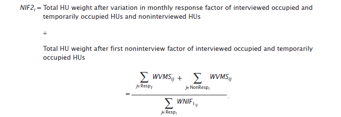
NIF1 weights for all occupied and temporarily occupied interviewed HUs are adjusted by this second noninterview factor. Vacant and deleted HUs are given a factor of 1.0, and noninterviews are assigned a factor of 0.0. The computation of the weight after the second noninterview adjustment factor is summarized in Table 11.7.
Footnote:
3Data are sorted by the weighting area, building type, and tabulation month. Within a building type, a tabulation month that has 10 or more responses is put in its own month. A tabulation month that has no nonresponses and some responses (even though the total is fewer than 10) is put in its own month. A tabulation month that has nonresponses and fewer than 10 responses is collapsed with the next month. If the final tabulation month needs to be collapsed, it is collapsed with the previous month.
Table 11.7 Computation of the Weight After the Second
Noninterview Adjustment Factor ( WNIF2 )
where
WNIF 2 ij = Adjusted HU weight after the second noninterview adjustment for the j th HU within the i th adjustment cell.
NIF1 weights for all occupied and temporarily occupied interviewed HUs are adjusted by this second noninterview factor. Vacant and deleted HUs are given a factor of 1.0, and noninterviews are assigned a factor of 0.0. The computation of the weight after the second noninterview adjustment factor is summarized in Table 11.7.
Footnote:
3Data are sorted by the weighting area, building type, and tabulation month. Within a building type, a tabulation month that has 10 or more responses is put in its own month. A tabulation month that has no nonresponses and some responses (even though the total is fewer than 10) is put in its own month. A tabulation month that has nonresponses and fewer than 10 responses is collapsed with the next month. If the final tabulation month needs to be collapsed, it is collapsed with the previous month.
Table 11.7 Computation of the Weight After the Second
Noninterview Adjustment Factor ( WNIF2 )
| Interview status | WNIF 2 ij |
|---|---|
| Occupied or temporarily occupied HU | WNIF 1 ij × NIF 2 i |
| Vacant or deleted HU | WNIFij |
| Noninterviewed HU | 0 |
where
WNIF 2 ij = Adjusted HU weight after the second noninterview adjustment for the j th HU within the i th adjustment cell.
One element not accounted for by the two noninterview factors above is the systematic differences that exist between characteristics of households that return census mail forms and those that do not (Weidman et al., 1995). The same element has been observed in the ACS across response modes. Virtually all noninterviews occur among the CAPI sample, and people in these HUs may have characteristics that are more similar to CAPI respondents than to mail and CATI respondents. Since the noninterview factors ( NIF1 and NIF2 ) are applied to all HUs interviewed by any mode, compensation may be needed for possible mode-related noninterview bias. The mode bias factor ensures that the total weights in the cells defined by a cross-classification of selected characteristics are the same as if the weight of noninterview HUs had been assigned only to CAPI HUs, but the factor distributes the weight across all respondents (within the cells) to reduce the effect on the variance of the resulting estimates.
The first step in the calculation of the mode bias noninterview factor ( MBF ) is to calculate an intermediate factor, referred to as the mode noninterview factor ( NIFM ). The NIFM is not used directly to compute an adjusted weight; instead, it is used as a factor applied to the WVMS weight to allow the calculation of the MBF . The cross-classification cells are defined for building type by tabulation month. Only HUs interviewed by CAPI and noninterviews are placed in the cells. If a cell contains fewer than 10 interviewed HUs, it is collapsed with an adjoining month. Cells with no noninterviews are never collapsed unless they are forced to collapse with a neighboring cell that fails the size criterion. The NIFM for a cell is:
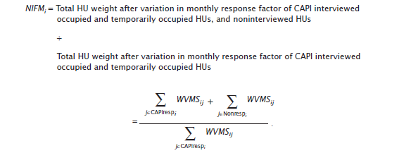
This mode noninterview factor is assigned to all CAPI-interviewed occupied and temporarily occupied HUs. HUs for which interviews are completed by mail or CATI, vacant HUs, and deleted HUs are given a factor of 1.0. Noninterviews are given a factor of 0.0. The NIFM factor is used in the next step only. Note that the NIFM adjustment is applied to the WVMS weight rather than the HU weight after the first and second noninterview adjustments ( WNIF1 and WNIF2 ). The computation of the weight after the mode noninterview adjustment factor is summarized in Table 11.8.
Table 11.8 Computation of the Weight After the Mode
Noninterview Adjustment Factor ( WNIFM )
where
WNIFMij = Adjusted HU weight after the mode noninterview adjustment for the j th HU within the i th adjustment cell.
Next, a cross-classification table is defined for tenure (three categories: HU owned, rented, or temporarily occupied), tabulation month (12 categories), and marital status of the householder (three categories: married/widowed, single, or unit is temporarily occupied). All occupied and temporarily occupied interviewed HUs are placed in their cells. If a cell has fewer than 10 interviewed HUs, the cells with the same tenure and month are collapsed across all marital statuses. If there are still fewer than 10 interviewed HUs, the cells with the same tenure are collapsed across all months. The mode bias factor ( MBF ) for each cell is then calculated as:
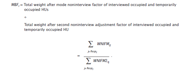
All interviewed occupied and temporarily occupied HUs are adjusted by this mode bias factor, and the remaining HUs receive the factor 1.0. These adjustments are applied to the WNIF2 weights. The computation of the weight after the mode bias factor is summarized in Table 11.9 below.
Table 11.9 Computation of the Weight After the Mode
Bias Factor ( WMBF )
where
WMBFij = Adjusted HU weight after the mode bias factor adjustment for the j th HU within the i th adjustment cell.
The first step in the calculation of the mode bias noninterview factor ( MBF ) is to calculate an intermediate factor, referred to as the mode noninterview factor ( NIFM ). The NIFM is not used directly to compute an adjusted weight; instead, it is used as a factor applied to the WVMS weight to allow the calculation of the MBF . The cross-classification cells are defined for building type by tabulation month. Only HUs interviewed by CAPI and noninterviews are placed in the cells. If a cell contains fewer than 10 interviewed HUs, it is collapsed with an adjoining month. Cells with no noninterviews are never collapsed unless they are forced to collapse with a neighboring cell that fails the size criterion. The NIFM for a cell is:
This mode noninterview factor is assigned to all CAPI-interviewed occupied and temporarily occupied HUs. HUs for which interviews are completed by mail or CATI, vacant HUs, and deleted HUs are given a factor of 1.0. Noninterviews are given a factor of 0.0. The NIFM factor is used in the next step only. Note that the NIFM adjustment is applied to the WVMS weight rather than the HU weight after the first and second noninterview adjustments ( WNIF1 and WNIF2 ). The computation of the weight after the mode noninterview adjustment factor is summarized in Table 11.8.
Table 11.8 Computation of the Weight After the Mode
Noninterview Adjustment Factor ( WNIFM )
| Interview status | WNIFMij |
|---|---|
| Occupied or temporarily occupied HU | WVMS 1 ij × NIFMi |
| Vacant or deleted HU | WVMSij |
| Noninterviewed HU | 0 |
where
WNIFMij = Adjusted HU weight after the mode noninterview adjustment for the j th HU within the i th adjustment cell.
Next, a cross-classification table is defined for tenure (three categories: HU owned, rented, or temporarily occupied), tabulation month (12 categories), and marital status of the householder (three categories: married/widowed, single, or unit is temporarily occupied). All occupied and temporarily occupied interviewed HUs are placed in their cells. If a cell has fewer than 10 interviewed HUs, the cells with the same tenure and month are collapsed across all marital statuses. If there are still fewer than 10 interviewed HUs, the cells with the same tenure are collapsed across all months. The mode bias factor ( MBF ) for each cell is then calculated as:
All interviewed occupied and temporarily occupied HUs are adjusted by this mode bias factor, and the remaining HUs receive the factor 1.0. These adjustments are applied to the WNIF2 weights. The computation of the weight after the mode bias factor is summarized in Table 11.9 below.
Table 11.9 Computation of the Weight After the Mode
Bias Factor ( WMBF )
| Interview status | WMBFij |
|---|---|
| Occupied or temporarily occupied HU | WNIF 2ij x MBFi |
| Vacant, deleted or noninterviewed HU | WNIF 2ij |
where
WMBFij = Adjusted HU weight after the mode bias factor adjustment for the j th HU within the i th adjustment cell.
This stage of weighting forces the ACS total HU and person weights to conform to estimates from the Census Bureau's PEP. The PEP of the Census Bureau annually produces estimates of population by sex, age, race, and Hispanic origin, and total HUs for each county in the United States as of July 1. The ACS estimates are based on a probability sample, and will vary from their true population values due to sampling and nonsampling error (see Chapters 12 and 14). In addition, we can see from the formulas for the adjustment factors in the previous two sections that the ACS estimates also will vary based on the combination of interviewed and noninterviewed HUs in each tabulation month. As part of the process of calculating person weights for the ACS, estimates of totals by sex, age, race, and Hispanic origin are controlled to be equal to population estimates by weighting area. There are two reasons for this: (1) to reduce the variability of the ACS HU and person estimates, and (2) to reduce bias due to under-coverage of HUs and the people within them in household surveys. The bias that results from missing these HUs and people is partly corrected by using these controls (Alexander et al., 1997).
The assignment of final weights involves the calculation of three factors based on the HU and population controls. The first adjustment involves the independent HU estimates. A second and separate adjustment relies on the independent population estimates. The final adjustment is implemented to achieve consistency between the ACS estimates of occupied HUs and householders.
The assignment of final weights involves the calculation of three factors based on the HU and population controls. The first adjustment involves the independent HU estimates. A second and separate adjustment relies on the independent population estimates. The final adjustment is implemented to achieve consistency between the ACS estimates of occupied HUs and householders.
The Census Bureau produces estimates of total HUs for states and counties as of July 1 on an annual basis. The estimates are computed based on a model:
HU0X = HU00 + (NC0X + NM0X) − HL0X
where the suffix "X" indicates the year of the HU estimates, and
HU0X = Estimated 200X HUs
HU00 = Geographically updated Census 2000 HUs
NC0X = Estimated residential construction, April 1, 2000, to July 1, 200X
NM0X = Estimated new residential mobile home placements, April 1, 2000, to July 1, 200X
HL0X = Estimated residential housing loss, April 1, 2000, to July 1, 200X.
For more detailed background on the current methodology used for the HU estimates, readers can visit
The Census Bureau also produces population estimates as of July 1 on an annual basis. Those estimates are computed based on the following simplified model:
P1 = P0 + B − D + NDM + NIM + NMM ,
where
P1 = population at the end of the period (current estimate year)
P0 = population at the beginning of the period (previous estimate year)
B = births during the period
D = deaths during the period
NDM = net domestic migration during the period
NIM = net international migration during the period
NMM = net military movement during the period.
In practice, the model is considerably more complex to leverage the best information available from multiple sources. For more detailed background on the current methodology used for the population estimates, readers can visit
Production of the population estimates for Puerto Rico is limited to population totals by municipio , and by sex-age distribution at the island level. For this reason, estimates of totals by municipio , sex, and age for the PRCS are controlled so as to be equal to the population estimates. Currently, there are no HU controls available for Puerto Rico.
Note that both HU and population estimates used as controls have a reference date of July 1 which means that the 12-month average of ACS characteristics is controlled to the population with the reference date of July 1. If person weights are controlled to the population estimates as of that date, it is logical that HUs also are controlled to those estimates to achieve a consistent relationship between the two totals.
The HU post-stratification factor is employed to adjust the estimated number of ACS HUs by weighting area to agree with the PEP estimates. For the i th weighting area, this factor ( HPF ) is:
HPFi = PEP HU estimate
÷
Total adjusted HU weight after the mode bias factor of interviewed occupied, interviewed temporarily
occupied, and vacant HUs
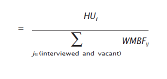
where
HUi = PEP housing unit estimate for the i th weighting area.
The denominator of the HPF formula aggregates the adjusted HU weight after the mode bias factor adjustment ( WMBF ) across 12 months for the interviewed occupied, interviewed temporarily occupied, and vacant HUs. All HUs then are adjusted by this HU post-stratification factor. Therefore, WHPF = WMBF × HPF , where WHPF is the adjusted HU weight after the HU post-stratification factor adjustment.
The HU post-stratification factor is employed to adjust the estimated number of ACS HUs by weighting area to agree with the PEP estimates. For the i th weighting area, this factor ( HPF ) is:
HPFi = PEP HU estimate
÷
Total adjusted HU weight after the mode bias factor of interviewed occupied, interviewed temporarily
occupied, and vacant HUs
where
HUi = PEP housing unit estimate for the i th weighting area.
The denominator of the HPF formula aggregates the adjusted HU weight after the mode bias factor adjustment ( WMBF ) across 12 months for the interviewed occupied, interviewed temporarily occupied, and vacant HUs. All HUs then are adjusted by this HU post-stratification factor. Therefore, WHPF = WMBF × HPF , where WHPF is the adjusted HU weight after the HU post-stratification factor adjustment.
The next step in the weighting process is to assign weights to persons via a three-dimensional raking-ratio estimation procedure. This is done so that (1) the combined estimates of spouses and unmarried partners conform to the combined estimate of married-couple and unmarried-partner households; (2) the estimate of householders conforms to the estimate of occupied housing units; and (3) the estimates for certain demographic groups are equal to their population estimates. Each person in an interviewed occupied HU is assigned an initial person weight equal to the HU weight after the HU post-stratification factor is applied ( WHPF ). Next, there are three steps of ratio adjustment. The first step uses three cells to classify persons by spousal or unmarried partner relationship to the householder. The second step uses two cells to classify persons by householder and nonhouseholder. The third step uses up to 156 cells defined by race/Hispanic origin, sex, and age. The steps are defined as follows:
Step 1: Spouses and Unmarried Partners. All persons are placed into one of three cells:
1. Persons who are the primary person in a two-partner relationship-all householders in a married-couple or unmarried-partner household.
2. Persons who are the secondary person in a two-partner relationship-all spouses or unmarried partners in those same households.
3. Balance of population-all persons not fitting into the first two cells.
The marginals for the first two cells are both equal to the estimate of married-couple plus unmarried-partner households using the WHPF weight. The marginal for the third cell is equal to the PEP total population estimate minus the sum of the marginals used for the other two cells. In this manner, the estimate of total population is controlled to the PEP total population estimate.
Step 2: Householders. The second step assigns all persons to one of two cells:
1.Householders
2.Nonhouseholders
The marginal for householders is the estimate of occupied HUs using the WHPF weight. The marginal for nonhouseholders is equal to the PEP total population estimate minus the marginal used for the first cell in order to control for total population.
Step 3: Race-Hispanic Origin/Sex/Age. The third step assigns all persons to one of up to 156 cells: six classifications of race-Hispanic origin by sex by 13 age groups. The marginals for these rows at the weighting area level come from the PEP population estimates. Some weighting areas will not have sufficient sample to support all 156 cells and in these cases some collapsing is necessary. This collapsing is done prior to the raking and remains fixed for all iterations of the raking.
Race and Hispanic origin are combined to define six unique race-ethnicity groups consistent with those used in weighting the Census 2000 long form. These groups are created by crossing "Non- Hispanic" with the five major single race groups, plus the group of all Hispanics regardless of race. The race-ethnicity groups are:
1. Non-Hispanic White
2. Non-Hispanic Black
3. Non-Hispanic American Indian and Alaska Native
4. Non-Hispanic Asian
5. Non-Hispanic Native Hawaiian or Pacific Islander
6. Hispanic
The assignment of a single major race to a person can be complicated because people can identify themselves as being of multiple races. People responding either with multiple races or "Other Race" are included in one of the six race-ethnicity groups for estimation purposes only. Subsequent ACS tabulations are based on the full set of responses to the race question.
Initial estimates of population totals are obtained from the ACS sample for each of the weighting race-ethnicity groups. These estimates are calculated based on the initial person weight of WHPF . Estimates from the Census Bureau's PEP also are available for each weighting race-ethnicity group. These total population estimates are used to control ACS total population estimates to be equal to the PEP by weighting area.
The initial sample and population estimates for each weighting race-ethnicity group are tested against a set of criteria that require a minimum of 10 sample people and a ratio of the population control to the initial sample estimate that is between (1/3.5) and 3.5. This is done to reduce the effect of large weights on the variance of the estimates. If there are weighting race-ethnicity groups that do not satisfy these requirements, they are collapsed until all groups satisfy the collapsing criteria. Collapsing decisions are made following a specified order in the following way (see Asiala, 2007, for further details):
1. If the requirements are not met when all non-Hispanic race groups are combined, then all weighting race-ethnicity groups are collapsed together and the collapsing is complete.
2. If the requirements are not met for Hispanics, the Hispanics are collapsed with the largest non-Hispanic non-White group.
3. If the requirements are not met for any non-Hispanic non-White group, it is collapsed with the largest (prior to collapsing) non-Hispanic non-White group.
4. If the largest collapsed non-Hispanic non-White group still does not meet the requirements, it is collapsed with the surviving non-Hispanic non-White groups in the following order until the requirements are met: Black, American Indian and Alaska Native, Asian, and Native Hawaiian or Pacific Islander.
5. If all non-Hispanic non-White groups have been collapsed together and the collapsed group still does not meet the requirements, it is collapsed with the non-Hispanic White group.
6. If the requirements are not met for the non-Hispanic White group, then it is collapsed with the largest non-Hispanic non-White group.
Within each collapsed weighting race-ethnicity group, the persons are placed in sex-age cells formed by crossing sex by the following 13 age categories: 0−4, 5−14, 15−17, 18−19, 20−24, 25−29, 30−34, 35−44, 45−49, 50−54, 55−64, 65−74, and 75+ years. If necessary, these cells also are collapsed to meet the requirements of the same sample size and a ratio between (1/3.5) and 3.5. The goals of the collapsing scheme are to keep children age 0−17 together whenever possible by first collapsing across sex within the first three age categories. In addition, the collapsing rules keep men age 18−54, women age 18−54, and seniors 55+ in separate groups by collapsing across age.
The initial sample cell estimates are then scaled and rescaled via iterative proportional fitting, or raking, so that the sum in each row or column consecutively agrees with the row or column household estimate (Steps 1 & 2) or population estimate (Step 3). This procedure is iterated a fixed number of times, and final person weights are assigned by applying an adjustment factor to the initial weights.
The scaling and rescaling between rows and columns is referred to as an iteration of raking. An iteration of raking consists of the following three steps. (The weighting matrix is included to facilitate the discussion below.) The three-step process has been split out into two tables, Table 11.10 and Table 11.11, for clarity.
Table 11.10 Steps 1 and 2 of the Weighting Matrix
Table 11.11 Steps 2 and 3 of the Weighting Matrix
Step 1. At this step, the initial person weights are adjusted to make both the sum of the weights of householders in married-couple or unmarried-partner households and the sum of the weights of their spouses or unmarried partners equal to the survey estimate of married-couple and unmarried-partner households. This is done using the HU weight after the HU post-stratification factor adjustment. The weights of all other persons are adjusted to make the sum of all weights equal to the PEP total population estimate.
Step 2. The Step 1 adjusted person weights are adjusted again to make the sum of the weights of all householders equal to the survey estimate of occupied HUs using the HU weight after the HU post-stratification factor adjustment. The Step 1 adjusted weights of all other persons are adjusted to make the sum of all weights equal to the total population estimate.
Step 3. The Step 2 adjusted person weights are adjusted a third time by the ratio of the population estimates of race-Hispanic origin/age/sex groups to the sum of the Step 2 weights for sample people in each of the demographic groups described previously.
The three steps of ratio adjustment are repeated in the order given above until the predefined stopping criterion is met. The stopping criterion is a function of the difference between Step 2 and Step 3 weights. The weights obtained from Step 3 of the final iteration are the final person weights.
A single factor, the person post-stratification factor ( PPSF ), is calculated at the person level, which captures the entire adjustment accomplished by the ratio-raking estimation. It is calculated as follows: PPSF = final person weight ÷ initial person weight.
The factor is calculated and applied to each person, so that their weights become the product of their initial weights and the factor.
ACS single-year estimates are produced for geographic areas with populations of at least 65,000, including incorporated places, for which population estimates also are published annually. Since population controls are applied at the weighting area level, occasionally the ACS estimate of total population for a large place within a weighting area may be far enough from its population estimate to cause confusion among data users. To avoid these anomalies, methodologies are being investigated to control person weights to total population for places with populations of at least 65,000 within weighting areas.
Step 1: Spouses and Unmarried Partners. All persons are placed into one of three cells:
1. Persons who are the primary person in a two-partner relationship-all householders in a married-couple or unmarried-partner household.
2. Persons who are the secondary person in a two-partner relationship-all spouses or unmarried partners in those same households.
3. Balance of population-all persons not fitting into the first two cells.
The marginals for the first two cells are both equal to the estimate of married-couple plus unmarried-partner households using the WHPF weight. The marginal for the third cell is equal to the PEP total population estimate minus the sum of the marginals used for the other two cells. In this manner, the estimate of total population is controlled to the PEP total population estimate.
Step 2: Householders. The second step assigns all persons to one of two cells:
1.Householders
2.Nonhouseholders
The marginal for householders is the estimate of occupied HUs using the WHPF weight. The marginal for nonhouseholders is equal to the PEP total population estimate minus the marginal used for the first cell in order to control for total population.
Step 3: Race-Hispanic Origin/Sex/Age. The third step assigns all persons to one of up to 156 cells: six classifications of race-Hispanic origin by sex by 13 age groups. The marginals for these rows at the weighting area level come from the PEP population estimates. Some weighting areas will not have sufficient sample to support all 156 cells and in these cases some collapsing is necessary. This collapsing is done prior to the raking and remains fixed for all iterations of the raking.
Race and Hispanic origin are combined to define six unique race-ethnicity groups consistent with those used in weighting the Census 2000 long form. These groups are created by crossing "Non- Hispanic" with the five major single race groups, plus the group of all Hispanics regardless of race. The race-ethnicity groups are:
1. Non-Hispanic White
2. Non-Hispanic Black
3. Non-Hispanic American Indian and Alaska Native
4. Non-Hispanic Asian
5. Non-Hispanic Native Hawaiian or Pacific Islander
6. Hispanic
The assignment of a single major race to a person can be complicated because people can identify themselves as being of multiple races. People responding either with multiple races or "Other Race" are included in one of the six race-ethnicity groups for estimation purposes only. Subsequent ACS tabulations are based on the full set of responses to the race question.
Initial estimates of population totals are obtained from the ACS sample for each of the weighting race-ethnicity groups. These estimates are calculated based on the initial person weight of WHPF . Estimates from the Census Bureau's PEP also are available for each weighting race-ethnicity group. These total population estimates are used to control ACS total population estimates to be equal to the PEP by weighting area.
The initial sample and population estimates for each weighting race-ethnicity group are tested against a set of criteria that require a minimum of 10 sample people and a ratio of the population control to the initial sample estimate that is between (1/3.5) and 3.5. This is done to reduce the effect of large weights on the variance of the estimates. If there are weighting race-ethnicity groups that do not satisfy these requirements, they are collapsed until all groups satisfy the collapsing criteria. Collapsing decisions are made following a specified order in the following way (see Asiala, 2007, for further details):
1. If the requirements are not met when all non-Hispanic race groups are combined, then all weighting race-ethnicity groups are collapsed together and the collapsing is complete.
2. If the requirements are not met for Hispanics, the Hispanics are collapsed with the largest non-Hispanic non-White group.
3. If the requirements are not met for any non-Hispanic non-White group, it is collapsed with the largest (prior to collapsing) non-Hispanic non-White group.
4. If the largest collapsed non-Hispanic non-White group still does not meet the requirements, it is collapsed with the surviving non-Hispanic non-White groups in the following order until the requirements are met: Black, American Indian and Alaska Native, Asian, and Native Hawaiian or Pacific Islander.
5. If all non-Hispanic non-White groups have been collapsed together and the collapsed group still does not meet the requirements, it is collapsed with the non-Hispanic White group.
6. If the requirements are not met for the non-Hispanic White group, then it is collapsed with the largest non-Hispanic non-White group.
Within each collapsed weighting race-ethnicity group, the persons are placed in sex-age cells formed by crossing sex by the following 13 age categories: 0−4, 5−14, 15−17, 18−19, 20−24, 25−29, 30−34, 35−44, 45−49, 50−54, 55−64, 65−74, and 75+ years. If necessary, these cells also are collapsed to meet the requirements of the same sample size and a ratio between (1/3.5) and 3.5. The goals of the collapsing scheme are to keep children age 0−17 together whenever possible by first collapsing across sex within the first three age categories. In addition, the collapsing rules keep men age 18−54, women age 18−54, and seniors 55+ in separate groups by collapsing across age.
The initial sample cell estimates are then scaled and rescaled via iterative proportional fitting, or raking, so that the sum in each row or column consecutively agrees with the row or column household estimate (Steps 1 & 2) or population estimate (Step 3). This procedure is iterated a fixed number of times, and final person weights are assigned by applying an adjustment factor to the initial weights.
The scaling and rescaling between rows and columns is referred to as an iteration of raking. An iteration of raking consists of the following three steps. (The weighting matrix is included to facilitate the discussion below.) The three-step process has been split out into two tables, Table 11.10 and Table 11.11, for clarity.
Table 11.10 Steps 1 and 2 of the Weighting Matrix
| Step 2 | Step 1 Control | |||
| Householder | Nonhouseholder | |||
| Step 1 | "Householder in two partner relationship" | "Survey estimate of married-couple and unmarried-partner households" | ||
| "Spouse/unmarried partner in two-partner relationship" | "Survey estimate of married-couple and unmarried-partner households" | |||
| Balance of population | "PEP total population estimate minus the sum of the two controls above" | |||
| Step 2 Control | "Survey estimate of occupied housing units" | "PEP total population estimate minus the control for householders" | ||
Table 11.11 Steps 2 and 3 of the Weighting Matrix
| Step 2 | Step 3 Control | ||||
| Householder | Nonhouseholder | ||||
| Step 3 | "Non-Hispanic White" | 0-4 Males | "PEP population estimate for the collapsed cell by weighting area" | ||
| 0-4 Females | |||||
| … | |||||
| 75+ Females | |||||
| Non-Hispanic AIAN | … | ||||
| Non-Hispanic Asian | … | ||||
| Non-Hispanic NHPI | … | ||||
| Hispanic | … | ||||
| Step 2 Control | "Survey estimate of occupied housing units" | "PEP total population estimate minus the control for householders" | |||
Step 1. At this step, the initial person weights are adjusted to make both the sum of the weights of householders in married-couple or unmarried-partner households and the sum of the weights of their spouses or unmarried partners equal to the survey estimate of married-couple and unmarried-partner households. This is done using the HU weight after the HU post-stratification factor adjustment. The weights of all other persons are adjusted to make the sum of all weights equal to the PEP total population estimate.
Step 2. The Step 1 adjusted person weights are adjusted again to make the sum of the weights of all householders equal to the survey estimate of occupied HUs using the HU weight after the HU post-stratification factor adjustment. The Step 1 adjusted weights of all other persons are adjusted to make the sum of all weights equal to the total population estimate.
Step 3. The Step 2 adjusted person weights are adjusted a third time by the ratio of the population estimates of race-Hispanic origin/age/sex groups to the sum of the Step 2 weights for sample people in each of the demographic groups described previously.
The three steps of ratio adjustment are repeated in the order given above until the predefined stopping criterion is met. The stopping criterion is a function of the difference between Step 2 and Step 3 weights. The weights obtained from Step 3 of the final iteration are the final person weights.
A single factor, the person post-stratification factor ( PPSF ), is calculated at the person level, which captures the entire adjustment accomplished by the ratio-raking estimation. It is calculated as follows: PPSF = final person weight ÷ initial person weight.
The factor is calculated and applied to each person, so that their weights become the product of their initial weights and the factor.
ACS single-year estimates are produced for geographic areas with populations of at least 65,000, including incorporated places, for which population estimates also are published annually. Since population controls are applied at the weighting area level, occasionally the ACS estimate of total population for a large place within a weighting area may be far enough from its population estimate to cause confusion among data users. To avoid these anomalies, methodologies are being investigated to control person weights to total population for places with populations of at least 65,000 within weighting areas.
Prior to the calculation of person weights, each HU has a single weight which is independent of the characteristics of the persons residing in the HU. After the calculation of person weights, a new HU weight is computed by taking into account the characteristics of the householder in the HU. In each interviewed occupied HU, the householder defined as the reference person (one of the persons who rents or owns the HU) is identified. Adjustment of the HU weight to account for the householder characteristics is done by assigning a householder factor ( HHF ) for an HU equal to the person post-stratification factor ( PPSF ) of the householder.4 Their PPSF s give an indication of under-coverage for households whose householders have the same demographic characteristics. The HHF adjustment uses this information to adjust for the resultant bias. Vacant HUs are given an HHF of 1.0 because they have no householders.
The adjusted HU weight accounting for householder characteristics is computed as a multiplication of the adjusted HU weight after the HU post-stratification factor adjustment ( WHPF ) with the householder factor ( HHF ). Therefore, WHHF = WHPF × HHF , where WHHF is the adjusted HU weight after the householder factor adjustment. The HU weight after the householder factor adjustment becomes the final HU weight.
The ACS weighting procedure results in two separate sets of weights, one for HUs and one for persons residing within HUs. However, since the housing unit weight is equal to the person weight of the householder, the survey will produce logically consistent estimates of occupied housing units, households, and householders. With this weighting procedure, the survey estimate of total housing units will differ slightly from the PEP total housing unit estimates. The difference between the ACS estimate the PEP estimate nationally, however, was less than 5,000 in 2006.
Footnote:
4In the calculation of person weights, the PPSF is used to adjust person weight so that the ACS population estimates conform to PEP estimates by demographic characteristics.
The multiyear estimation methodology involves reweighting the data for each sample address in the 3- or 5-year period and is not just a simple average of the single-year estimates. The weighting methodology for the multiyear estimation is very similar to the methodology used for the single-year weighting. Thus, only the differences between the single- and multiyear weighting are described in this section.
The data for all sample addresses over the multiyear period are pooled together into one file. The single-year base weights are then adjusted by the reciprocal of the number of years in the period so that each year contributes its proportional share to the multiyear estimates. For example, for the 2005−2007 3-year weighting, the base weights are all divided by three.
The interview month assigned to each address is also recoded so that all the data from the entire period appears as though it came from a 1-year period. For example, in the 2005−2007 3-year weighting, all addresses that were originally assigned an interview month of January 2005, 2006, or 2007 are assigned the common interview month of January. Thus, when the weighting is performed, those records will all be treated as though they come from the same month for the VMS , NIF2 , NIFM , and MBF adjustments. By pooling the records across years in this manner, the noninterview adjustments, in particular, require less collapsing because of the larger sample in each cell. This, in turn, should better preserve the seasonal trends that may be present in the population as captured by the ACS.
The interview month assigned to each address is also recoded so that all the data from the entire period appears as though it came from a 1-year period. For example, in the 2005−2007 3-year weighting, all addresses that were originally assigned an interview month of January 2005, 2006, or 2007 are assigned the common interview month of January. Thus, when the weighting is performed, those records will all be treated as though they come from the same month for the VMS , NIF2 , NIFM , and MBF adjustments. By pooling the records across years in this manner, the noninterview adjustments, in particular, require less collapsing because of the larger sample in each cell. This, in turn, should better preserve the seasonal trends that may be present in the population as captured by the ACS.
The geography for all sample addresses in the period are updated into the common geography of the final year. This allows the tabulation of the data to be in a consistent, constant geography that is the most recent and likely most relevant to data users. When tabulating estimates for an area, all interviews from the period that are considered to be inside the boundaries of that area in the final year of the period will be included in the estimates regardless if they were considered to be inside the boundaries for that area at the time of interview. As a by-product of this methodology, the ACS is also able to publish multiyear estimates for newly created places or counties that did not exist when the interviews for the addresses in that place or county were collected.
Since the multiyear estimate is an estimate for the period, the controls are not those of a particular year but rather they are the average of the annual independent population estimates over the period. The PEP refreshes their entire time series of estimates going back to the previous census each year using the most current data and methodology. Each of these time series are considered a "vintage." In order for the ACS to make use of the best available population estimates as controls, the multiyear weighting uses the population estimates of the most recent vintage for all years in the period in order to derive the multiyear controls.
These derived estimates are created for the HU, GQs population, and total population for use as controls in the multiyear weighting. The derived county-level HU estimates are the simple average across all years in the period. Since the average is typically not an integer, the result is rounded to the final integerized estimate. Likewise, the derived GQ population estimates for state by major type group are the simple average across all years in the period. Those averages are then control rounded so that the rounded state average estimate is within one of the unrounded estimate. Finally, the derived total population estimates by race, ethnicity, age, and sex are averaged across all years in the period and control rounded to form the final derived estimates. This is done prior to the collapsing of the estimates into the 156 cells per weighting area needed for the demographic dimension of the household person weighting as described in the single-year person weighting section.
These derived estimates are created for the HU, GQs population, and total population for use as controls in the multiyear weighting. The derived county-level HU estimates are the simple average across all years in the period. Since the average is typically not an integer, the result is rounded to the final integerized estimate. Likewise, the derived GQ population estimates for state by major type group are the simple average across all years in the period. Those averages are then control rounded so that the rounded state average estimate is within one of the unrounded estimate. Finally, the derived total population estimates by race, ethnicity, age, and sex are averaged across all years in the period and control rounded to form the final derived estimates. This is done prior to the collapsing of the estimates into the 156 cells per weighting area needed for the demographic dimension of the household person weighting as described in the single-year person weighting section.
Once the data are pooled and put into the geography of the final year, they are weighted using the single-year weighting methodology through the MBF adjustment. It is after this adjustment that the only weighting step specific to the multiyear weighting methodology is implemented, the model-assisted estimation procedure. An earlier research project (Starsinic, 2005) compared the variances of ACS tract-level estimates formed from the 1999−2001 ACS to the variances of the Census 2000 long-form estimates. The results of that research showed that the variances of the ACS tract-level estimates were higher in relation to the long form than what we expected based on sample size alone. The primary source of that increased variance was attributed to the lack of ACS subcounty controls at the tract-level or lower as was used for the long form.
Several options were explored on how the ACS estimates of variance for subcounty estimates might be improved. One option considered was to use the ACS sampling frame counts as subcounty controls. Other options explored ways to create subcounty population controls, including tract-level population controls. The final approach, and the one that was chosen, introduces a model-assisted estimation step into the multiyear weighting that makes use of both the sampling frame counts and administrative records to reduce the level of variance in the subcounty estimates (Fay, 2006). An important feature of the model-assisted estimation procedure is that the administrative record data is not used directly to produce ACS estimates. The administrative record data are only used to help reduce the level of variance. The published ACS estimates are still formed from weighted totals of the ACS survey data.
The entire model-assisted estimation process is summarized in these steps:
1. Create frame counts for places and Minor Civil Divisions (MCDs) that contain at least 10,000 in population and at least 300 HU addresses (the 5-year estimation will use tracts simply satisfying the latter criterion).
2. Link the administrative records to the ACS sampling frame (the Master Address File [MAF]) and drop administrative records that cannot be linked.
3. Form unweighted place- and MCD-level totals (tract-level for the 5-year estimates) of the linked administrative record characteristics.
4. Apply the WMBF weights at the HU level to the linked administrative records that fall into the ACS sample. The weighted estimates at this step represent (essentially) unbiased estimates of the unweighted totals in Step 2.
5. Using generalized regression estimation, fit a model to calibrate the ACS weights so that the weighted totals from the linked ACS records match the unweighted totals from Step 2 and so that the weighted ACS estimate of HUs match the frame totals in Step 1. The categories of the variables considered in the regression are collapsed or removed as necessary to fit a good model.
6. Proceed with the remaining steps of the ACS weighting starting with the Housing Unit Poststratification (HPF) Factor adjustments, including the person weighting using the derived multiyear controls as described in the preceding section.
The BWs , which reflect the sampling probabilities of selection, should sum to the count of records on the sampling frame at the county and, generally, the subcounty level. However, after the noninterview adjustments the weighted subcounty distribution of the interviewed sample cases can deviate from the original frame distribution. This can impact both the subcounty estimates and the variances on those estimates. The use of frame counts as subcounty controls reestablishes the original distribution of HU addresses on the frame in the weighted sample. For the 3-year weighting, these frame counts are calculated at the place- or MCD-level. If the place or MCD has a PEP population estimate of 10,000 or more then the ACS weights are controlled to those frame counts at that subcounty level. For the 5-year weighting, these frame counts will be computed for tracts. This control to the frame counts is the simplest model and is used if a model with administrative record data cannot be estimated. Otherwise, it is one part of the entire calibration performed in this step.
The administrative record data used for this step is created from linking two primary files maintained by the Data Integration Division at the Census Bureau. The first file includes person characteristics and has been created from a combination of social security and census information. The second file uses administrative records to identify all possible addresses of the persons on the first file. A merged file is then created which contains only the age, sex, race, and Hispanic origin of each person and an identifier that links that person to the best address available in the MAF via a Master Address File ID (MAFID). No other characteristics or publicly identifiable information are present on the file. This file is updated annually to account for new births, death information, and for updated address information.
For each MAFID, it is possible to create household demographic totals of people by age/sex and race/ethnicity from the merged administrative records for each address that is matched to the MAF. The age/sex totals are calculated within seven categories:
1. All persons age 0−17
2. All persons age 18−29
3. Males age 30−44
4. Females age 30−44
5. Males age 45−64
6. Females age 45−64
7. All persons age 65 and older
The race/ethnicity totals are calculated within four categories:
1. All Hispanics regardless of race
2. All non-Hispanic Blacks
3. All non-Hispanic Whites
4. All non-Hispanics other races
These household-level totals can then be used to create unweighted place- and MCD-level administrative record universe totals using the geography associated with the address.
The administrative records that match to the sampling frame can also be linked to the actual ACS sample records themselves. Using the WMBF weights, the records that match to the ACS sample can then be used to create weighted administrative record totals for the same geographic areas. Since the ACS sample weights should reflect the frame counts, these weighted administrative record totals should be an unbiased estimate of the unweighted universe totals.
Using generalized regression estimation (or GREG), the ACS weights are first calibrated so that the weighted administrative record totals match the unweighted universe counts for the seven age/sex categories. Two conditions are checked: is the regression equation solvable and are all of the resulting weights greater than 0.5? If either condition fails then the age/sex categories are collapsed and the regression is attempted again. Two levels of collapsing are attempted:
1. Collapsing across age/sex categories into three categories: all persons age 0−17, all persons age 18−44, and all persons 45 and older.
2. Collapsing all categories into a single cell of total administrative persons.
The alternative: do not make use of the administrative record data. If the regression passes using at least the single cell of total administrative persons, then an attempt is made to add the race/ethnicity covariates to the model. First, a collapsing procedure is run that tests which race/ethnicity categories can be used. The criteria for including a race/ethnicity category in the regression is that both the administrative records universe count for the category being tested and the total for all other categories must be greater than 300 persons. This procedure is carried out first for the largest race/ethnicity category not including the non- Hispanic White category, then the next largest such category, and finally the last remaining category other than non-Hispanic White.
As an example, if the largest category other than non-Hispanic White was the Hispanic category, then the first test would be if (1) the Hispanic category had a universe count which was greater than 300 and (2) the other three categories combined had a universe count greater than 300. If it passes, the Hispanic category is flagged for inclusion and the remaining categories are tested. If the next largest category is non-Hispanic Black, it is tested to determine if its universe count is greater than 300 and if the balance, now only the non-Hispanic other races and non-Hispanic White, is greater than 300. If it passes, then the procedure moves on to test the smallest category other than non-Hispanic White. In this example, that is the non-Hispanic other race category. If a similar test on that category fails (or on any previous attempt) then the race collapsing is complete and the covariates for each race/ethnicity category that passed are added to the model. The regression is then attempted including both the age/sex and race/ethnicity covariates. The same conditions used in the age/sex category collapsing are applied to the new attempt. If the regression passes both conditions then the covariate matrix is considered final. If the regression fails either condition, then the smallest race/ethnicity category is not included in the model and the regression is attempted again. This process continues until either the regression passes or all race/ethnicity covariates have been removed.
Apply the GREG Weighting Factor (GWTF): The final result of this step is the creation of the GWTF for each ACS record, which captures the calibration performed in the regression. A summary of the impact of the GWTF is given in Table 11.12.able 11.12
Table 11.12: Impact of GREG Weighting Factor Adjustment
This factor is then applied to the WMBF weights to create the weight after the GREG Weighting Factor (WGWTF). The computation of this weight is summarized in Table 11.13.
Table 11.13 Computation of the Weight After the GREG
Weighting Factor
After this step is complete, the multiyear weighting mirrors the single-year weighting, picking up again at the HPF step.
1. Collapsing across age/sex categories into three categories: all persons age 0−17, all persons age 18−44, and all persons 45 and older.
2. Collapsing all categories into a single cell of total administrative persons.
The alternative: do not make use of the administrative record data. If the regression passes using at least the single cell of total administrative persons, then an attempt is made to add the race/ethnicity covariates to the model. First, a collapsing procedure is run that tests which race/ethnicity categories can be used. The criteria for including a race/ethnicity category in the regression is that both the administrative records universe count for the category being tested and the total for all other categories must be greater than 300 persons. This procedure is carried out first for the largest race/ethnicity category not including the non- Hispanic White category, then the next largest such category, and finally the last remaining category other than non-Hispanic White.
As an example, if the largest category other than non-Hispanic White was the Hispanic category, then the first test would be if (1) the Hispanic category had a universe count which was greater than 300 and (2) the other three categories combined had a universe count greater than 300. If it passes, the Hispanic category is flagged for inclusion and the remaining categories are tested. If the next largest category is non-Hispanic Black, it is tested to determine if its universe count is greater than 300 and if the balance, now only the non-Hispanic other races and non-Hispanic White, is greater than 300. If it passes, then the procedure moves on to test the smallest category other than non-Hispanic White. In this example, that is the non-Hispanic other race category. If a similar test on that category fails (or on any previous attempt) then the race collapsing is complete and the covariates for each race/ethnicity category that passed are added to the model. The regression is then attempted including both the age/sex and race/ethnicity covariates. The same conditions used in the age/sex category collapsing are applied to the new attempt. If the regression passes both conditions then the covariate matrix is considered final. If the regression fails either condition, then the smallest race/ethnicity category is not included in the model and the regression is attempted again. This process continues until either the regression passes or all race/ethnicity covariates have been removed.
Apply the GREG Weighting Factor (GWTF): The final result of this step is the creation of the GWTF for each ACS record, which captures the calibration performed in the regression. A summary of the impact of the GWTF is given in Table 11.12.able 11.12
Table 11.12: Impact of GREG Weighting Factor Adjustment
| Interview status | and the ACS record is: | Impact of GWTF |
|---|---|---|
| Not applicable | No impact (factor set to 1) |
| " In and out-of-scope place/ MCD that has either insufficient population or frame counts" | No impact (factor set to 1) |
| "In an in-scope place/MCD but does not match to administrative data or the model using administrative data fails" | "Adjusts weights to calibrate to frame counts for the area" |
| "In an in-scope place/MCD, matches to the administrative data and the model using administrative data passes" | "Adjusts weights to calibrate to frame counts and calibrate weighted administrative data to administrative universe counts " |
This factor is then applied to the WMBF weights to create the weight after the GREG Weighting Factor (WGWTF). The computation of this weight is summarized in Table 11.13.
Table 11.13 Computation of the Weight After the GREG
Weighting Factor
| Interview status | WGWTFj |
|---|---|
| Interview or field determined ineligible housing unit | WMBFj × GWTFj |
| All others= | 0 |
After this step is complete, the multiyear weighting mirrors the single-year weighting, picking up again at the HPF step.
In addition to the adjustments to the single-year weighting methodology for weighting the multiyear data, there are other steps involved in the multiyear estimation that are not weighting related. These include standardizing definitions of variables, updating the geography for place of work and migration characteristics, and the adjustment of income, value, and other dollar amounts for inflation over the period. The details of these adjustments are given in Chapter 10.
Alexander, C., S. Dahl, and L. Weidman. (1997). " Making Estimates From the American Community Survey." JSM Proceedings, Social Statistics Section , Alexandria, VA: American Statistical Association, pp. 88−97. .
Asiala, M. (2007). "Specifications for Weighting the ACS 2006 HU Sample (ACS06-W-5)." 2006 American Community Survey Weighting Memorandum Series #ACS06-W-5, June 27, 2007 Draft Census Bureau Memorandum to S. Schechter Bortner from D. Whitford, Washington, DC: U.S. Census Bureau.
Fay, R. (2006). "Using Administrative Records With Model-Assisted Estimation for the American Community Survey." JSM Proceedings, Survey Research Methods Section , Alexandria, VA: American Statistical Association, pp. 2995−3001.
Starsinic, M. (2005). "American Community Survey: Improving Reliability for Small Area Estimates." JSM Proceedings, Survey Research Methods Section , Alexandria, VA: American Statistical Association, pp. 3592−3599.
U.S. Census Bureau (2007). Methodology: Housing Unit Estimates (2006), Washington, DC: U.S. Census Bureau,
U.S. Census Bureau (2008). "Methodology: State and Count Population Estimates (2007)," Washington, DC: U.S. Census Bureau.
Weidman, L., C. Alexander, G. Diffendahl, and S. Love. (1995). "Estimation Issues for the Continuous Measurement Survey." JSM Proceedings, Survey Research Methods Section , Alexandria, VA: American Statistical Association, pp. 596−601..
Weidman, L., M. Ikeda, and J. Tsay. (2007). "Comparison of Alternatives for Controlling Group Quarters Person Estimates in the American Community Survey," Statistical Research Division Research Series RRS2007-4, Washington, DC: U.S. Census Bureau.
Asiala, M. (2007). "Specifications for Weighting the ACS 2006 HU Sample (ACS06-W-5)." 2006 American Community Survey Weighting Memorandum Series #ACS06-W-5, June 27, 2007 Draft Census Bureau Memorandum to S. Schechter Bortner from D. Whitford, Washington, DC: U.S. Census Bureau.
Fay, R. (2006). "Using Administrative Records With Model-Assisted Estimation for the American Community Survey." JSM Proceedings, Survey Research Methods Section , Alexandria, VA: American Statistical Association, pp. 2995−3001.
Starsinic, M. (2005). "American Community Survey: Improving Reliability for Small Area Estimates." JSM Proceedings, Survey Research Methods Section , Alexandria, VA: American Statistical Association, pp. 3592−3599.
U.S. Census Bureau (2007). Methodology: Housing Unit Estimates (2006), Washington, DC: U.S. Census Bureau,
U.S. Census Bureau (2008). "Methodology: State and Count Population Estimates (2007)," Washington, DC: U.S. Census Bureau.
Weidman, L., C. Alexander, G. Diffendahl, and S. Love. (1995). "Estimation Issues for the Continuous Measurement Survey." JSM Proceedings, Survey Research Methods Section , Alexandria, VA: American Statistical Association, pp. 596−601.
Weidman, L., M. Ikeda, and J. Tsay. (2007). "Comparison of Alternatives for Controlling Group Quarters Person Estimates in the American Community Survey," Statistical Research Division Research Series RRS2007-4, Washington, DC: U.S. Census Bureau.

