


| Documentation: | ACS 2008 (3-Year Estimates) |
you are here:
choose a survey
survey
document
chapter
Publisher: U.S. Census Bureau
Survey: ACS 2008 (3-Year Estimates)
| Document: | ACS 2008-3yr Summary File: Technical Documentation |
| citation: | Social Explorer; U.S. Census Bureau; American Community Survey 2006-2008 Summary File: Technical Documentation. |
Chapter Contents
The accuracy of the data documents provides data users with a basic understanding of the sample design, confidentiality, sampling error, nonsampling error, estimation methodology, and accuracy of the data.
Revised January 25, 2010
The data contained in these data products are based on the American Community Survey (ACS) sample interviewed from January 1, 2008 through December 31, 2008. The ACS sample is selected from all counties and county-equivalents in the United States. In 2006, the ACS began collection of data from sampled persons in group quarters (GQs) - for example, military barracks, college dormitories, nursing homes, and correctional facilities. Persons in group quarters are included with persons in housing units (HUs) in all 2008 ACS estimates that are based on the total population. All ACS population estimates from years prior to 2006 include only persons in housing units. The ACS, like any other statistical activity, is subject to error. The purpose of this documentation is to provide data users with a basic understanding of the ACS sample design, estimation methodology, and accuracy of the ACS data. The ACS is sponsored by the U.S. Census Bureau, and is part of the 2010 Decennial Census Program. Additional information on the operational aspects of the ACS, including data collection and processing, can be found in the Design and Methodology: ACS Report.
The ACS employs three modes of data collection:
Month 1: Addresses in sample that are determined to be mailable are sent a questionnaire via the U.S. Postal Service.
Month 2: All mail non-responding addresses with an available phone number are sent to CATI.
Month 3: A sample of mail non-responses without a phone number, CATI non-responses, and unmailable addresses are selected and sent to CAPI.
Note that mail responses are accepted during all three months of data collection. All Remote Alaska addresses are assigned to one of two data collection periods, January-April, or September-December and are sampled for CAPI at a rate of 2-in-3. Data for these addresses are collected using CAPI only and up to four months are given to complete the interviews in Remote Alaska for each data collection period.
- Mailout/Mailback
- Computer Assisted Telephone Interview (CATI)
- Computer Assisted Personal Interview (CAPI)
Month 1: Addresses in sample that are determined to be mailable are sent a questionnaire via the U.S. Postal Service.
Month 2: All mail non-responding addresses with an available phone number are sent to CATI.
Month 3: A sample of mail non-responses without a phone number, CATI non-responses, and unmailable addresses are selected and sent to CAPI.
Note that mail responses are accepted during all three months of data collection. All Remote Alaska addresses are assigned to one of two data collection periods, January-April, or September-December and are sampled for CAPI at a rate of 2-in-3. Data for these addresses are collected using CAPI only and up to four months are given to complete the interviews in Remote Alaska for each data collection period.
Group Quarters data collection spans six weeks, except in Remote Alaska and for Federal prisons, where the data collection time period is four months. As is done for HUs, Group Quarters in Remote Alaska are assigned to one of two data collection periods, January-April, or September-December and up to four months is allowed to complete the interviews. Similarly, all Federal prisons are assigned to September with a four month data collection window.
Field representatives have several options available to them for data collection. These include completing the questionnaire while speaking to the resident in person or over the telephone, conducting a personal interview with a proxy, such as a relative or guardian, or leaving paper questionnaires for residents to complete for themselves and then pick them up later. This last option is used for data collection in Federal prisons.
Field representatives have several options available to them for data collection. These include completing the questionnaire while speaking to the resident in person or over the telephone, conducting a personal interview with a proxy, such as a relative or guardian, or leaving paper questionnaires for residents to complete for themselves and then pick them up later. This last option is used for data collection in Federal prisons.
The universe for the ACS consists of all valid, residential housing unit addresses in all county and county equivalents in the 50 states, including the District of Columbia. The Master Address File (MAF) is a database maintained by the Census Bureau containing a listing of residential and commercial addresses in the U.S. and Puerto Rico. The MAF is updated twice each year with the Delivery Sequence Files (DSF) provided by the U.S. Postal Service. The DSF covers only the U.S. These files identify mail drop points and provide the best available source of changes and updates to the housing unit inventory. The MAF is also updated with the results from various Census Bureau field operations, including the ACS.
The group quarters (GQ) sampling frame is created from the Special Place (SP)/GQ facility files, obtained from decennial census operations, merged with the MAF. This frame includes GQs added from operations such as the GQ Incomplete Information Operation (IIO) at the Census Bureau's National Processing Center in Jeffersonville, Indiana, the Census Questionnaire Resolution (CQR) Program and GQs closed on Census day. The GQ frame also underwent an unduplication process. GQs that were closed on Census day were not included in the SP/GQ inventory file received from Decennial Systems and Contract Management Office (DSCMO). These were added from a preliminary inventory file obtained from DSCMO since it was possible that while these GQs were closed on Census day, they could be open when the ACS contacts them. Headquarters Staff researched state prisons on the Internet to obtain the current operating status and the current population counts for state prisons. After the frame was put together from these different sources, it was then sorted geographically.
The ACS employs a two-phase, two-stage sample design. The ACS first-phase sample consists of two separate samples, Main and Supplemental, each chosen at different points in time. Together, these constitute the first-phase sample. Both the Main and the Supplemental samples are chosen in two stages referred to as first- and second-stage sampling. Subsequent to second stage sampling, sample addresses are randomly assigned to one of the twelve months of the sample year. The second-phase of sampling occurs when the CAPI sample is selected (see Section 2 below).
The Main sample is selected during the summer preceding the sample year. Approximately 99 percent of the sample is selected at this time. Each address in sample is randomly assigned to one of the 12 months of the sample year. Supplemental sampling occurs in January/February of the sample year and accounts for approximately 1 percent of the overall first-phase sample. The Supplemental sample is allocated to the last nine months of the sample year. A sub-sample of non-responding addresses and of any addresses deemed unmailable is selected for the CAPI data collection mode.
Several of the steps used to select the first-phase sample are common to both Main and Supplemental sampling. The descriptions of the steps included in the first-phase sample selection below indicate which are common to both and which are unique to either Main or Supplemental sampling.
1. First-phase Sample Selection
For American Indian, Tribal Subdivisions, and Alaska Native Village Statistical Areas, the measure of size is the estimated number of occupied HUs multiplied by the proportion of people reporting American Indian or Alaska Native (alone or in combination) in Census 2000.
Each block is then assigned the smallest measure of size from the set of all entities of which it is a part. The second-stage sampling strata and the overall first-phase sampling rates are shown in Table 1 below.
These rates also account for expected growth of the HU inventory between Main and Supplemental of roughly 1 percent. The first-phase rates are adjusted for the first-stage sample to yield the second-stage selection probabilities.
Table 1. First-phase Sampling Rate Categories for the United States
1MOS = Measure of size.
2TRACTMOS = Census Tract measure of size.
3Mailable addresses: Addresses that have sufficient information to be delivered by the U.S. Postal Service (as determined by ACS).
2. Second-phase Sample Selection - Subsampling the Unmailable and Non-Responding Addresses All addresses determined to be unmailable are subsampled for the CAPI phase of data collection at a rate of 2-in-3. Unmailable addresses, which include Remote Alaska addresses, do not go to the CATI phase of data collection. Subsequent to CATI, all addresses for which no response has been obtained prior to CAPI are subsampled based on the expected rate of completed interviews at the tract level using the rates shown in Table 2.
Table 2. Second-Phase (CAPI) Subsampling Rates for the United States
The Main sample is selected during the summer preceding the sample year. Approximately 99 percent of the sample is selected at this time. Each address in sample is randomly assigned to one of the 12 months of the sample year. Supplemental sampling occurs in January/February of the sample year and accounts for approximately 1 percent of the overall first-phase sample. The Supplemental sample is allocated to the last nine months of the sample year. A sub-sample of non-responding addresses and of any addresses deemed unmailable is selected for the CAPI data collection mode.
Several of the steps used to select the first-phase sample are common to both Main and Supplemental sampling. The descriptions of the steps included in the first-phase sample selection below indicate which are common to both and which are unique to either Main or Supplemental sampling.
1. First-phase Sample Selection
- First-stage sampling (performed during both Main and Supplemental sampling)
- Assignment of blocks to a second-stage sampling stratum ( performed during Main sampling only)
- Counties
- Places
- School Districts (elementary, secondary, and unified)
- American Indian Areas
- Tribal Subdivisions
- Alaska Native Village Statistical Areas
- Hawaiian Homelands
- Minor Civil Divisions - in Connecticut, Maine, Massachusetts, Michigan, Minnesota, New Hampshire, New Jersey, New York, Pennsylvania, Rhode Island, Vermont, and Wisconsin (these are the states where MCDs are active, functioning governmental units)
- Census Designated Places - in Hawaii only
For American Indian, Tribal Subdivisions, and Alaska Native Village Statistical Areas, the measure of size is the estimated number of occupied HUs multiplied by the proportion of people reporting American Indian or Alaska Native (alone or in combination) in Census 2000.
Each block is then assigned the smallest measure of size from the set of all entities of which it is a part. The second-stage sampling strata and the overall first-phase sampling rates are shown in Table 1 below.
- Calculation of the second-stage sampling rates (performed during Main sampling only )
These rates also account for expected growth of the HU inventory between Main and Supplemental of roughly 1 percent. The first-phase rates are adjusted for the first-stage sample to yield the second-stage selection probabilities.
- Second-stage sample selection (performed in Main and Supplemental )
- Sample Month Assignment ( performed in Main and Supplemental )
Table 1. First-phase Sampling Rate Categories for the United States
| Sampling Rate Category | Sampling Rates |
|---|---|
| Blocks in smallest governmental units (MOS1 < 200) | 10.0% |
| Blocks in smaller governmental units (200 ≤ MOS < 800) | 6.6% |
| Blocks in small governmental units (800 ≤ MOS ≤ 1200) | 3.3% |
| Blocks in large tracts(MOS >1200, TRACTMOS2 ≥ 2000) where Mailable addresses3 ≥ 75% and predicted levels of completed mail and CATI interviews prior tosecond-stage sampling > 60% | 1.49% |
| Other Blocks in large tracts (MOS >1200, TRACTMOS ≥ 2000)All other blocks | 1.62% |
| (MOS >1200, TRACTMOS < 2000) where Mailable addresses ≥ 75% and predicted levels of completed mailand CATI interviews prior to second-stage sampling > 60% | 2.02% |
| All other blocks (MOS >1200, TRACTMOS < 2000) | 2.2% |
1MOS = Measure of size.
2TRACTMOS = Census Tract measure of size.
3Mailable addresses: Addresses that have sufficient information to be delivered by the U.S. Postal Service (as determined by ACS).
2. Second-phase Sample Selection - Subsampling the Unmailable and Non-Responding Addresses All addresses determined to be unmailable are subsampled for the CAPI phase of data collection at a rate of 2-in-3. Unmailable addresses, which include Remote Alaska addresses, do not go to the CATI phase of data collection. Subsequent to CATI, all addresses for which no response has been obtained prior to CAPI are subsampled based on the expected rate of completed interviews at the tract level using the rates shown in Table 2.
Table 2. Second-Phase (CAPI) Subsampling Rates for the United States
| Address and Tract Characteristics | CAPI Subsampling Rate |
|---|---|
| United States | |
| Unmailable addresses and addresses in Remote AlaskaMailable addresses in tracts with predicted levels of completed | 66.7% |
| mail and CATI interviews prior to CAPI subsampling between 0%and less than 36%Mailable addresses in tracts with predicted levels of completed | 50% |
| mail and CATI interviews prior to CAPI subsampling greater than35% and less than 51% | 40% |
| Mailable addresses in other tracts | 33.3% |
The GQ sampling frame is divided into three strata: one for small GQs (having 15 or fewer people according to Census 2000 or updated information), one for GQs that were closed on Census Day 2000, and one for large GQs (having more than 15 people according to Census 2000 or updated information). GQs in the first two strata are sampled using the same procedure, and GQs in the large stratum are sampled using different a method. The small GQ stratum and the stratum for GQs closed on Census Day are combined into one sampling stratum and sorted geographically 1.
1. First-phase Sample Selection for Small GQ Stratum
Footnote:
1Note that all references to the small GQ stratum include both small GQs and GQs closed on Census day.
2. Sample Selection for the Large GQ Stratum
Unlike housing unit address sampling and the small GQ sample selection, the large GQ sampling procedure has no first-stage in which sampling units are randomly assigned to one of five years. All large GQs are eligible for sampling each year. The large GQ samples are selected using a two-phase design.
First-phase Sampling
In the large GQ stratum, GQ hits are selected using a systematic PPS (probability proportional to size) sample, with a target sampling rate that varies according to state. A hit refers to a grouping of 10 expected interviews. GQs are selected with probability proportional to its most current count of persons or capacity. For stratification, and for sampling the large GQs, a GQ measure of size (GQMOS) is computed, where GQMOS is the expected population of the GQ divided by 10. This reflects that the GQ data is collected in groups of 10 GQ persons. People are selected in hits of 10 in a systematic sample of 1-in-x where x = 1 rate (1 divided by the states target sampling rate). For example, suppose a state had a target sampling rate of 2.5%. The hits would then be selected in a systematic sample of 1-in-40, since 1 0.025 = 40. The following table summarizes the 2008 state targeted sampling rates for the U.S.
Table 3. 2008 State Targeted Sampling Rates for the U.S.
All GQs in this stratum are eligible for sampling every year, regardless of their sample status in previous years. For large GQs, hits can be selected multiple times in the sample year. For most GQ types, the hits are randomly assigned throughout the year. Some GQs may have multiple hits with the same sample date if more than 12 hits are selected from the GQ. In these cases, the person sample within that month is unduplicated.
3. Sample Month Assignment
In order to assign a panel month to each hit, all of the GQ samples from a state are combined and sorted by small/large stratum and second-phase order of selection. Consecutive samples are assigned to the twelve panel months in a predetermined order, starting with a randomly determined month, except for Federal prisons and remote Alaska. Remote Alaska GQs are assigned to January and September based on where the GQ is located. Correctional facilities have their sample clustered. All Federal prisons hits are assigned to the September panel. In non-Federal correctional facilities, all hits for a given GQ are assigned to the same panel month. However, unlike Federal prisons, the hits in state and local correctional facilities are assigned to randomly selected panels spread throughout the year.
4. Second Phase Sample: Selection of Persons in Small and Large GQs
Small GQs in the second phase sampling are "take all," i.e., every person in the selected GQ is eligible to receive a questionnaire. If the actual number of persons in the GQ exceeds 15, a field subsampling operation is performed to reduce the total number of sample persons interviewed at the GQ to 10. If the actual number of persons in the GQ is 10 or fewer, then the group size will be less than 10.
For each hit in the large GQs, the automated instrument uses the population count at the time of the visit and selects a subsample of 10 people from the roster. The people in this subsample receive the questionnaire.
1. First-phase Sample Selection for Small GQ Stratum
- First-stage sampling
- Second-stage sampling
Footnote:
1Note that all references to the small GQ stratum include both small GQs and GQs closed on Census day.
2. Sample Selection for the Large GQ Stratum
Unlike housing unit address sampling and the small GQ sample selection, the large GQ sampling procedure has no first-stage in which sampling units are randomly assigned to one of five years. All large GQs are eligible for sampling each year. The large GQ samples are selected using a two-phase design.
First-phase Sampling
In the large GQ stratum, GQ hits are selected using a systematic PPS (probability proportional to size) sample, with a target sampling rate that varies according to state. A hit refers to a grouping of 10 expected interviews. GQs are selected with probability proportional to its most current count of persons or capacity. For stratification, and for sampling the large GQs, a GQ measure of size (GQMOS) is computed, where GQMOS is the expected population of the GQ divided by 10. This reflects that the GQ data is collected in groups of 10 GQ persons. People are selected in hits of 10 in a systematic sample of 1-in-x where x = 1 rate (1 divided by the states target sampling rate). For example, suppose a state had a target sampling rate of 2.5%. The hits would then be selected in a systematic sample of 1-in-40, since 1 0.025 = 40. The following table summarizes the 2008 state targeted sampling rates for the U.S.
Table 3. 2008 State Targeted Sampling Rates for the U.S.
| Alaska | 5.53% | New Hampshire | 3.17% |
| Delaware | 4.86% | New Mexico | 3.06% |
| District of Columbia | 3.08% | North Dakota | 4.59% |
| Hawaii | 3.24% | Rhode Island | 2.75% |
| Idaho | 3.48% | South Dakota | 3.91% |
| Maine | 3.14% | Utah | 2.79% |
| Montana | 4.38% | Vermont | 4.95% |
| Nevada | 3.36% | Wyoming | 7.11% |
| All Other States | 2.50% | ||
All GQs in this stratum are eligible for sampling every year, regardless of their sample status in previous years. For large GQs, hits can be selected multiple times in the sample year. For most GQ types, the hits are randomly assigned throughout the year. Some GQs may have multiple hits with the same sample date if more than 12 hits are selected from the GQ. In these cases, the person sample within that month is unduplicated.
3. Sample Month Assignment
In order to assign a panel month to each hit, all of the GQ samples from a state are combined and sorted by small/large stratum and second-phase order of selection. Consecutive samples are assigned to the twelve panel months in a predetermined order, starting with a randomly determined month, except for Federal prisons and remote Alaska. Remote Alaska GQs are assigned to January and September based on where the GQ is located. Correctional facilities have their sample clustered. All Federal prisons hits are assigned to the September panel. In non-Federal correctional facilities, all hits for a given GQ are assigned to the same panel month. However, unlike Federal prisons, the hits in state and local correctional facilities are assigned to randomly selected panels spread throughout the year.
4. Second Phase Sample: Selection of Persons in Small and Large GQs
Small GQs in the second phase sampling are "take all," i.e., every person in the selected GQ is eligible to receive a questionnaire. If the actual number of persons in the GQ exceeds 15, a field subsampling operation is performed to reduce the total number of sample persons interviewed at the GQ to 10. If the actual number of persons in the GQ is 10 or fewer, then the group size will be less than 10.
For each hit in the large GQs, the automated instrument uses the population count at the time of the visit and selects a subsample of 10 people from the roster. The people in this subsample receive the questionnaire.
The estimates that appear in this product are obtained from a raking ratio estimation procedure that results in the assignment of two sets of weights: a weight to each sample person record and a weight to each sample housing unit record. Estimates of person characteristics are based on the person weight. Estimates of family, household, and housing unit characteristics are based on the housing unit weight. For any given tabulation area, a characteristic total is estimated by summing the weights assigned to the persons, households, families or housing units possessing the characteristic in the tabulation area. Each sample person or housing unit record is assigned exactly one weight to be used to produce estimates of all characteristics. For example, if the weight given to a sample person or housing unit has a value 40, all characteristics of that person or housing unit are tabulated with the weight of 40.
The weighting is conducted in two main operations: a group quarters person weighting operation which assigns weights to persons in group quarters, and a household person weighting operation which assigns weights both to housing units and to persons within housing units. The group quarters person weighting is conducted first and the household person weighting second. The household person weighting is dependent on the group quarters person weighting because estimates for total population which include both group quarters and household population are controlled to the Census Bureau's official 2008 total resident population estimates.
The weighting is conducted in two main operations: a group quarters person weighting operation which assigns weights to persons in group quarters, and a household person weighting operation which assigns weights both to housing units and to persons within housing units. The group quarters person weighting is conducted first and the household person weighting second. The household person weighting is dependent on the group quarters person weighting because estimates for total population which include both group quarters and household population are controlled to the Census Bureau's official 2008 total resident population estimates.
Each GQ person is first assigned to a Population Estimates Program Major GQ Type Group (the type groups used by the Population Estimates Program). The major type groups used are:
Table 3: Population Estimates Program Major GQ Type Groups
The procedure used to assign the weights to the GQ persons is performed independently within state. The steps are as follows:
State x Major GQ Type Group x County
The GQ person post-stratification factor is computed and assigned using the following groups:
State x Major GQ Type Group
Major GQ Type Group
Major GQ Type Group x County
Housing Unit and Household Person Weighting
The housing unit and household person weighting use weighting areas built from collections of whole counties. Census 2000 data are used to group counties of similar demographic and social characteristics. The characteristics considered in the formation include:
The estimation procedure used to assign the weights is then performed independently within each of the ACS weighting areas.
1. Initial Housing Unit Weighting Factors-This process produced the following factors:
Selected in CAPI subsampling: SSF = 2.0, 2.5, or 3.0 according to Table 2
Not selected in CAPI subsampling: SSF = 0.0
Not a CAPI case: SSF = 1.0
Some sample addresses are unmailable. A two-thirds sample of these is sent directly to CAPI and for these cases SSF = 1.5.
This factor makes the total weight of the Mail, CATI, and CAPI records to be tabulated in a month equal to the total base weight of all cases originally mailed for that month. For all cases, VMS is computed and assigned based on the following groups:
Weighting Area x Month
Weighting Area x Building Type x Tract
A second factor, NIF2, is a ratio adjustment that is computed and assigned to occupied housing units based on the following groups:
Weighting Area x Building Type x Month
NIF is then computed by applying NIF1 and NIF2 for each occupied housing unit. Vacant housing units are assigned a value of NIF = 1.0. Nonresponding housing units are now assigned a weight of 0.0.
Weighting Area x Building Type (single or multi unit) x Month
Vacant housing units or non-CAPI (mail and CATI) housing units receive a value of NIFM = 1.0.
This factor makes the total weight of the housing units in the groups below the same as if NIFM had been used instead of NIF. MBF is computed and assigned to occupied housing units based on the following groups: Weighting Area x Tenure (owner or renter) x Month x Marital Status of the Householder (married/widowed or single)
Vacant housing units receive a value of MBF = 1.0. MBF is applied to the weights computed through NIF.
2. Person Weighting Factors-Initially the person weight of each person in an occupied housing unit is the product of the weighting factors of their associated housing unit (BW x ... x HPF). At this point everyone in the household has the same weight. Beginning in 2006, the person weighting is done in a series of three steps which are repeated until a stopping criterion is met. These three steps form a raking ratio or raking process. These person weights are individually adjusted for each person as described below.
The three steps are as follows:
Householder in a married-couple or unmarried-partner household
Spouse or unmarried partner in a married-couple or unmarried-partner household
All others
The first two groups are adjusted so that the sum of their person weights is equal to the total estimate of married-couple or unmarried-partner households using the housing unit weight (BW x ... x HPF). The goal of this step is to produce more consistent estimates of spouses or unmarried partners and married-couple and unmarried-partner households.
Householders
Non-householders
The first group is adjusted so that the sum of their person weights is equal to the total estimate of occupied housing units using the housing unit weight (BW x ... x HPF). The goal of this step is to produce more consistent estimates of householders, occupied housing units, and households.
Weighting Area x Race / Ethnicity (non-Hispanic White, non-Hispanic
Black, non-Hispanic American Indian or Alaskan Native, non-Hispanic
Asian, non-Hispanic Native Hawaiian or Pacific Islander, and Hispanic
(any race)) x Sex x Age Groups.
These three steps are repeated several times until the estimates at the national level achieve their optimal consistency with regard to the spouse and householder equalization. The effect Person Post-Stratification Factor (PPSF) is then equal to the product (SPEQRF x HHEQRF x DEMORF) from all of iterations of these three adjustments. The unrounded person weight is then the equal to the product of PPSF times the housing unit weight (BW x ... x HPF x PPSF).
3. Rounding-The final product of all person weights (BW x ... x HPF x PPSF) is rounded to an integer. Rounding is performed so that the sum of the rounded weights is within one person of the sum of the unrounded weights for any of the groups listed below:
County
County x Race
County x Race x Hispanic Origin
County x Race x Hispanic Origin x Sex
County x Race x Hispanic Origin x Sex x Age
County x Race x Hispanic Origin x Sex x Age x Tract
County x Race x Hispanic Origin x Sex x Age x Tract x Block
For example, the number of White, Hispanic, Males, Age 30 estimated for a county using the rounded weights is within one of the number produced using the unrounded weights.
4. Final Housing Unit Weighting Factors-This process produces the following factors:
County
County x Tract
County x Tract x Block
Table 3: Population Estimates Program Major GQ Type Groups
| Major GQ Type Group | Definition | Institutional / Non-Institutional |
|---|---|---|
| 1 | Correctional Institutions | Institutional |
| 2 | Juvenile Detention Facilities | Institutional |
| 3 | Nursing Homes | Institutional |
| 4 | Other Long-Term Care Facilities | Institutional |
| 5 | College Dormitories | Non-Institutional |
| 6 | Military Facilities | Non-Institutional |
| 7 | Other Non-Institutional Facilities | Non-Institutional |
- Base Weight
- Non-Interview Factor
State x Major GQ Type Group x County
- GQ Person Post-stratification Factor
The GQ person post-stratification factor is computed and assigned using the following groups:
State x Major GQ Type Group
- Rounding
Major GQ Type Group
Major GQ Type Group x County
Housing Unit and Household Person Weighting
The housing unit and household person weighting use weighting areas built from collections of whole counties. Census 2000 data are used to group counties of similar demographic and social characteristics. The characteristics considered in the formation include:
- Percent in poverty
- Percent renting
- Percent in rural areas
- Race, ethnicity, age, and sex distribution
- Distance between the centroids of the counties
- Core-based Statistical Area status
The estimation procedure used to assign the weights is then performed independently within each of the ACS weighting areas.
1. Initial Housing Unit Weighting Factors-This process produced the following factors:
- Base Weight (BW)
- CAPI Subsampling Factor (SSF)
Selected in CAPI subsampling: SSF = 2.0, 2.5, or 3.0 according to Table 2
Not selected in CAPI subsampling: SSF = 0.0
Not a CAPI case: SSF = 1.0
Some sample addresses are unmailable. A two-thirds sample of these is sent directly to CAPI and for these cases SSF = 1.5.
- Variation in Monthly Response by Mode (VMS)
This factor makes the total weight of the Mail, CATI, and CAPI records to be tabulated in a month equal to the total base weight of all cases originally mailed for that month. For all cases, VMS is computed and assigned based on the following groups:
Weighting Area x Month
- Noninterview Factor (NIF)
Weighting Area x Building Type x Tract
A second factor, NIF2, is a ratio adjustment that is computed and assigned to occupied housing units based on the following groups:
Weighting Area x Building Type x Month
NIF is then computed by applying NIF1 and NIF2 for each occupied housing unit. Vacant housing units are assigned a value of NIF = 1.0. Nonresponding housing units are now assigned a weight of 0.0.
- Noninterview Factor-Mode (NIFM)
Weighting Area x Building Type (single or multi unit) x Month
Vacant housing units or non-CAPI (mail and CATI) housing units receive a value of NIFM = 1.0.
- Mode Bias Factor (MBF)
This factor makes the total weight of the housing units in the groups below the same as if NIFM had been used instead of NIF. MBF is computed and assigned to occupied housing units based on the following groups: Weighting Area x Tenure (owner or renter) x Month x Marital Status of the Householder (married/widowed or single)
Vacant housing units receive a value of MBF = 1.0. MBF is applied to the weights computed through NIF.
- Housing unit Post-stratification Factor (HPF)
2. Person Weighting Factors-Initially the person weight of each person in an occupied housing unit is the product of the weighting factors of their associated housing unit (BW x ... x HPF). At this point everyone in the household has the same weight. Beginning in 2006, the person weighting is done in a series of three steps which are repeated until a stopping criterion is met. These three steps form a raking ratio or raking process. These person weights are individually adjusted for each person as described below.
The three steps are as follows:
- Spouse Equalization Raking Factor (SPEQRF)
Householder in a married-couple or unmarried-partner household
Spouse or unmarried partner in a married-couple or unmarried-partner household
All others
The first two groups are adjusted so that the sum of their person weights is equal to the total estimate of married-couple or unmarried-partner households using the housing unit weight (BW x ... x HPF). The goal of this step is to produce more consistent estimates of spouses or unmarried partners and married-couple and unmarried-partner households.
- Householder Equalization Raking Factor (HHEQRF)
Householders
Non-householders
The first group is adjusted so that the sum of their person weights is equal to the total estimate of occupied housing units using the housing unit weight (BW x ... x HPF). The goal of this step is to produce more consistent estimates of householders, occupied housing units, and households.
- Demographic Raking Factor (DEMORF)
Weighting Area x Race / Ethnicity (non-Hispanic White, non-Hispanic
Black, non-Hispanic American Indian or Alaskan Native, non-Hispanic
Asian, non-Hispanic Native Hawaiian or Pacific Islander, and Hispanic
(any race)) x Sex x Age Groups.
These three steps are repeated several times until the estimates at the national level achieve their optimal consistency with regard to the spouse and householder equalization. The effect Person Post-Stratification Factor (PPSF) is then equal to the product (SPEQRF x HHEQRF x DEMORF) from all of iterations of these three adjustments. The unrounded person weight is then the equal to the product of PPSF times the housing unit weight (BW x ... x HPF x PPSF).
3. Rounding-The final product of all person weights (BW x ... x HPF x PPSF) is rounded to an integer. Rounding is performed so that the sum of the rounded weights is within one person of the sum of the unrounded weights for any of the groups listed below:
County
County x Race
County x Race x Hispanic Origin
County x Race x Hispanic Origin x Sex
County x Race x Hispanic Origin x Sex x Age
County x Race x Hispanic Origin x Sex x Age x Tract
County x Race x Hispanic Origin x Sex x Age x Tract x Block
For example, the number of White, Hispanic, Males, Age 30 estimated for a county using the rounded weights is within one of the number produced using the unrounded weights.
4. Final Housing Unit Weighting Factors-This process produces the following factors:
- Householder Factor (HHF)
- Rounding
County
County x Tract
County x Tract x Block
The Census Bureau has modified or suppressed some data on this site to protect confidentiality. Title 13 United States Code, Section 9, prohibits the Census Bureau from publishing results in which an individual's data can be identified.
The Census Bureau's internal Disclosure Review Board sets the confidentiality rules for all data releases. A checklist approach is used to ensure that all potential risks to the confidentiality of the data are considered and addressed.
The Census Bureau's internal Disclosure Review Board sets the confidentiality rules for all data releases. A checklist approach is used to ensure that all potential risks to the confidentiality of the data are considered and addressed.
- Title 13, United States Code
- Disclosure Avoidance
- Data Swapping
- Synthetic Data
- Sampling Error
- Nonsampling Error
Sampling error is the difference between an estimate based on a sample and the corresponding value that would be obtained if the estimate were based on the entire population (as from a census). Note that sample-based estimates will vary depending on the particular sample selected from the population. Measures of the magnitude of sampling error reflect the variation in the estimates over all possible samples that could have been selected from the population using the same sampling methodology.
Estimates of the magnitude of sampling errors - in the form of margins of error - are provided with all published ACS data. The Census Bureau recommends that data users incorporate this information into their analyses, as sampling error in survey estimates could impact the conclusions drawn from the results.
Estimates of the magnitude of sampling errors - in the form of margins of error - are provided with all published ACS data. The Census Bureau recommends that data users incorporate this information into their analyses, as sampling error in survey estimates could impact the conclusions drawn from the results.
Confidence Intervals - A sample estimate and its estimated standard error may be used to construct confidence intervals about the estimate. These intervals are ranges that will contain the average value of the estimated characteristic that results over all possible samples, with a known probability.
For example, if all possible samples that could result under the ACS sample design were independently selected and surveyed under the same conditions, and if the estimate and its estimated standard error were calculated for each of these samples, then:
1. Approximately 68 percent of the intervals from one estimated standard error below the estimate to one estimated standard error above the estimate would contain the average result from all possible samples;
2. Approximately 90 percent of the intervals from 1.645 times the estimated standard error below the estimate to 1.645 times the estimated standard error above the estimate would contain the average result from all possible samples.
3. Approximately 95 percent of the intervals from two estimated standard errors below the estimate to two estimated standard errors above the estimate would contain the average result from all possible samples.
The intervals are referred to as 68 percent, 90 percent, and 95 percent confidence intervals, respectively.
Margin of Error - Instead of providing the upper and lower confidence bounds in published ACS tables, the margin of error is provided instead. The margin of error is the difference between an estimate and its upper or lower confidence bound. Both the confidence bounds and the standard error can easily be computed from the margin of error. All ACS published margins of error are based on a 90 percent confidence level.
Standard Error = Margin of Error / 1.645
Lower Confidence Bound = Estimate - Margin of Error
Upper Confidence Bound = Estimate + Margin of Error
Note that for 2005 and earlier estimates, ACS margins of error and confidence bounds were calculated using a 90 percent confidence level multiplier of 1.65. Beginning with the 2006 data release, we are now employing a more accurate multiplier of 1.645. Margins of error and confidence bounds from previously published products will not be updated with the new multiplier. When calculating standard errors from margins of error or confidence bounds using published data for 2005 and earlier, use the 1.65 multiplier.
When constructing confidence bounds from the margin of error, the user should be aware of any "natural" limits on the bounds. For example, if a population estimate is near zero, the calculated value of the lower confidence bound may be negative. However, a negative number of people does not make sense, so the lower confidence bound should be reported as zero instead. However, for other estimates such as income, negative values do make sense. The context and meaning of the estimate must be kept in mind when creating these bounds. Another of these natural limits would be 100 percent for the upper bound of a percent estimate.
If the margin of error is displayed as ' *****' (five asterisks), the estimate has been controlled to be equal to a fixed value and so it has no sampling error. When using any of the formulas in the following section, use a standard error of zero for these controlled estimates. Limitations -The user should be careful when computing and interpreting confidence intervals.
The estimated standard errors (and thus margins of error) included in these data products do not include portions of the variability due to nonsampling error that may be present in the data. In particular, the standard errors do not reflect the effect of correlated errors introduced by interviewers, coders, or other field or processing personnel. Nor do they reflect the error from imputed values due to missing responses. Thus, the standard errors calculated represent a lower bound of the total error. As a result, confidence intervals formed using these estimated standard errors may not meet the stated levels of confidence (i.e., 68, 90, or 95 percent). Thus, some care must be exercised in the interpretation of the data in this data product based on the estimated standard errors.
Zero or small estimates; very large estimates - The value of almost all ACS characteristics is greater than or equal to zero by definition. For zero or small estimates, use of the method given previously for calculating confidence intervals relies on large sample theory, and may result in negative values which for most characteristics are not admissible. In this case the lower limit of the confidence interval is set to zero by default. A similar caution holds for estimates of totals close to control total or estimated proportions near one, where the upper limit of the confidence interval is set to its largest admissible value. In these situations the level of confidence of the adjusted range of values is less than the prescribed confidence level.
Direct estimates of the standard errors were calculated for all estimates reported in this product. The standard errors, in most cases, are calculated using a replicate-based methodology that takes into account the sample design and estimation procedures. Excluding the base weights, replicate weights were allowed to be negative in order to avoid underestimating the standard error.
Exceptions include:
1. The estimate of the number or proportion of people, households, families, or housing units in a geographic area with a specific characteristic is zero. A special procedure is used to estimate the standard error.
2. There are either no sample observations available to compute an estimate or standard error of a median, an aggregate, a proportion, or some other ratio, or there are too few sample observations to compute a stable estimate of the standard error. The estimate is represented in the tables by "-" and the margin of error by '**' (two asterisks).
3. The estimate of a median falls in the lower open-ended interval or upper open-ended interval of a distribution. If the median occurs in the lowest interval, then a "-" follows the estimate, and if the median occurs in the upper interval, then a "+" follows the estimate. In both cases the margin of error is represented in the tables by '***' (three asterisks).
Sums and Differences of Direct Standard Errors - The standard errors estimated from these tables are for individual estimates. Additional calculations are required to estimate the standard errors for sums of and differences between two sample estimates. The estimate of the standard error of a sum or difference is approximately the square root of the sum of the two individual standard errors squared; that is, for standard errors ) SE( X ˆ) and SE of estimates (Y ˆ SE X ˆ andY ˆ) :
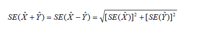
This method, however, will underestimate (overestimate) the standard error if the two items in a sum are highly positively (negatively) correlated or if the two items in a difference are highly negatively (positively) correlated.
Ratios - The statistic of interest may be the ratio of two estimates. First is the case where the numerator is not a subset of the denominator. The standard error of this ratio between two sample estimates is approximated as:

Proportions/percents - For a proportion (or percent), a ratio where the numerator is a subset of the denominator, a slightly different estimator is used. Note the difference between the formulas for the standard error for proportions (below) and ratios (above) - the plus sign in the previous formula has been replaced with a minus sign. If the value under the square root sign is negative, use the ratio standard error formula above, instead. If Pˆ =Xˆ /Yˆ , then
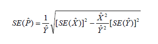
If Qˆ = 100%´ Pˆ (P is the proportion and Q is its corresponding percent), then SE(Qˆ ) = 100%´ SE(Pˆ) .
Products - For a product of two estimates - for example if you want to estimate a proportions numerator by multiplying the proportion by its denominator - the standard error can be approximated as

Significant differences - Users may conduct a statistical test to see if the difference between an ACS estimate and any other chosen estimates is statistically significant at a given confidence level. "Statistically significant" means that the difference is not likely due to random chance alone. With the two estimates (Est1 and Est2) and their respective standard errors (SE1 and SE2), calculate

If Z > 1.645 or Z < -1.645, then the difference can be said to be statistically significant at the 90 percent confidence level. [Note that we are now recommending that +/-1.645 be used to determine significance. Previous ACS Accuracy of the Data documents suggested using +/- 1.65.] Any estimate can be compared to an ACS estimate using this method, including other ACS estimates from the current year, the ACS estimate for the same characteristic and geographic area but from a previous year, Census 2000 100 percent counts and long form estimates, estimates from other Census Bureau surveys, and estimates from other sources. Not all estimates have sampling error - Census 2000 100 percent counts do not, for example, although Census 2000 long form estimates do - but they should be used if they exist to give the most accurate result of the test.
Users are also cautioned to not rely on looking at whether confidence intervals for two estimates overlap to determine statistical significance, because there are circumstances where that method will not give the correct test result. The Z calculation above is recommended in all cases. All statistical testing in ACS data products is based on the 90 percent confidence level. Users should understand that all testing was done using unrounded estimates and standard errors, and it may not be possible to replicate test results using the rounded estimates and margins of error as published.
Exceptions include:
1. The estimate of the number or proportion of people, households, families, or housing units in a geographic area with a specific characteristic is zero. A special procedure is used to estimate the standard error.
2. There are either no sample observations available to compute an estimate or standard error of a median, an aggregate, a proportion, or some other ratio, or there are too few sample observations to compute a stable estimate of the standard error. The estimate is represented in the tables by "-" and the margin of error by '**' (two asterisks).
3. The estimate of a median falls in the lower open-ended interval or upper open-ended interval of a distribution. If the median occurs in the lowest interval, then a "-" follows the estimate, and if the median occurs in the upper interval, then a "+" follows the estimate. In both cases the margin of error is represented in the tables by '***' (three asterisks).
Sums and Differences of Direct Standard Errors - The standard errors estimated from these tables are for individual estimates. Additional calculations are required to estimate the standard errors for sums of and differences between two sample estimates. The estimate of the standard error of a sum or difference is approximately the square root of the sum of the two individual standard errors squared; that is, for standard errors ) SE( X ˆ) and SE of estimates (Y ˆ SE X ˆ andY ˆ) :
This method, however, will underestimate (overestimate) the standard error if the two items in a sum are highly positively (negatively) correlated or if the two items in a difference are highly negatively (positively) correlated.
Ratios - The statistic of interest may be the ratio of two estimates. First is the case where the numerator is not a subset of the denominator. The standard error of this ratio between two sample estimates is approximated as:
Proportions/percents - For a proportion (or percent), a ratio where the numerator is a subset of the denominator, a slightly different estimator is used. Note the difference between the formulas for the standard error for proportions (below) and ratios (above) - the plus sign in the previous formula has been replaced with a minus sign. If the value under the square root sign is negative, use the ratio standard error formula above, instead. If Pˆ =Xˆ /Yˆ , then
If Qˆ = 100%´ Pˆ (P is the proportion and Q is its corresponding percent), then SE(Qˆ ) = 100%´ SE(Pˆ) .
Products - For a product of two estimates - for example if you want to estimate a proportions numerator by multiplying the proportion by its denominator - the standard error can be approximated as
Significant differences - Users may conduct a statistical test to see if the difference between an ACS estimate and any other chosen estimates is statistically significant at a given confidence level. "Statistically significant" means that the difference is not likely due to random chance alone. With the two estimates (Est1 and Est2) and their respective standard errors (SE1 and SE2), calculate
If Z > 1.645 or Z < -1.645, then the difference can be said to be statistically significant at the 90 percent confidence level. [Note that we are now recommending that +/-1.645 be used to determine significance. Previous ACS Accuracy of the Data documents suggested using +/- 1.65.] Any estimate can be compared to an ACS estimate using this method, including other ACS estimates from the current year, the ACS estimate for the same characteristic and geographic area but from a previous year, Census 2000 100 percent counts and long form estimates, estimates from other Census Bureau surveys, and estimates from other sources. Not all estimates have sampling error - Census 2000 100 percent counts do not, for example, although Census 2000 long form estimates do - but they should be used if they exist to give the most accurate result of the test.
Users are also cautioned to not rely on looking at whether confidence intervals for two estimates overlap to determine statistical significance, because there are circumstances where that method will not give the correct test result. The Z calculation above is recommended in all cases. All statistical testing in ACS data products is based on the 90 percent confidence level. Users should understand that all testing was done using unrounded estimates and standard errors, and it may not be possible to replicate test results using the rounded estimates and margins of error as published.
We will present some examples based on the real data to demonstrate the use of the formulas.
Example 1 - Calculating the Standard Error from the Confidence Interval The estimated number of males, never married is 41,011,718 from summary table B12001 for the United States for 2008. The margin of error is 93,906.
Standard Error = Margin of Error / 1.645
Calculating the standard error using the margin of error, we have:
SE(41,011,718) = 93,906 / 1.645 = 57,086.
Example 2 - Calculating the Standard Error of a Sum
We are interested in the number of people who have never been married. From Example 1, we know the number of males, never married is 41,011,718. From summary table B12001 we have the number of females, never married is 34,893,327 with a margin of error of 81,141. So, the estimated number of people who have never been married is 41,011,718 + 34,893,327 = 75,905,045. To calculate the standard error of this sum, we need the standard errors of the two estimates in the sum. We have the standard error for the number of males never married from example 1 as 57,086. The standard error for the number of females never married is calculated using the margin of error:
SE(34,893,327) = 81,141 / 1.645 = 49,326.
So using the formula for the standard error of a sum or difference we have: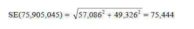
Caution: This method, however, will underestimate (overestimate) the standard error if the two items in a sum are highly positively (negatively) correlated or if the two items in a difference are highly negatively (positively) correlated.
To calculate the lower and upper bounds of the 90 percent confidence interval around 75,905,045 using the standard error, simply multiply 75,444 by 1.645, then add and subtract the product from 75,905,045. Thus the 90 percent confidence interval for this estimate is [75,905,045 - 1.645(75,444)] to [75,905,045 + 1.645(75,444)] or 75,780,940 to 76,029,150.
Example 3 - Calculating the Standard Error of a Proportion/Percent
We are interested in the percentage of females who have never been married to the number of people who have never been married. The number of females, never married is 34,893,327 and the number of people who have never been married is 75,905,045. To calculate the standard error of this proportion or percent, we need the standard errors of the two estimates in the proportion. We have the standard error for the number of females never married from example 2 as 49,326 and the standard error for the number of people never married calculated from example 2 as 75,444.
The estimate is (34,893,327 / 75,905,045) * 100% = 45.97%
So, using the formula for the standard error of a proportion or percent, we have:
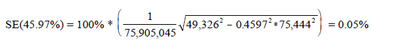
To calculate the lower and upper bounds of the 90 percent confidence interval around 45.97 using the standard error, simply multiply 0.05 by 1.645, then add and subtract the product from 45.97. Thus the 90 percent confidence interval for this estimate is [45.97 - 1.645(0.05)] to [45.97 + 1.645(0.05)], or 45.89% to 46.05%.
Example 4 - Calculating the Standard Error of a Ratio
Now, let us calculate the estimate of the ratio of the number of unmarried males to the number of unmarried females and its standard error. From the above examples, the estimate for the number of unmarried men is 41,011,718 with a standard error of 57,086, and the estimate for the number of unmarried women is 34,893,327 with a standard error of 49,326.
The estimate of the ratio is 41,011,718 / 34,893,327 = 1.175.
The standard error of this ratio is

The 90 percent margin of error for this estimate would be 0.00233 multiplied by 1.645, or about 0.004. The 90 percent lower and upper 90 percent confidence bounds would then be [1.175 - 0.004] to [1.175 + 0.004], or 1.171 and 1.179.
Example 5 - Calculating the Standard Error of a Product
We are interested in the number of 1-unit detached owner-occupied housing units. The number of owner-occupied housing units is 75,373,053 with a margin of error of 224,087 from subject table S2504 for 2008, and the percent of 1-unit detached owner-occupied housing units is 81.8% (0.818) with a margin of error of 0.1 (0.001). So the number of 1- unit detached owner-occupied housing units is 75,373,053 * 0.818 = 61,655,157. Calculating the standard error for the estimates using the margin of error we have:
SE(75,373,053) = 224,087 / 1.645 = 136,223 and SE(0.818) = 0.001 / 1.645 = 0.0006079
The standard error for number of 1-unit detached owner-occupied housing units is calculated using the formula for products as:
To calculate the lower and upper bounds of the 90 percent confidence interval around 61,655,157 using the standard error, simply multiply 120,483 by 1.645, then add and subtract the product from 61,655,157. Thus the 90 percent confidence interval for this estimate is [61,655,157 - 1.645(120,483)] to [61,655,157 + 1.645(120,483)] or 61,456,962 to 61,853,352.
Example 1 - Calculating the Standard Error from the Confidence Interval The estimated number of males, never married is 41,011,718 from summary table B12001 for the United States for 2008. The margin of error is 93,906.
Standard Error = Margin of Error / 1.645
Calculating the standard error using the margin of error, we have:
SE(41,011,718) = 93,906 / 1.645 = 57,086.
Example 2 - Calculating the Standard Error of a Sum
We are interested in the number of people who have never been married. From Example 1, we know the number of males, never married is 41,011,718. From summary table B12001 we have the number of females, never married is 34,893,327 with a margin of error of 81,141. So, the estimated number of people who have never been married is 41,011,718 + 34,893,327 = 75,905,045. To calculate the standard error of this sum, we need the standard errors of the two estimates in the sum. We have the standard error for the number of males never married from example 1 as 57,086. The standard error for the number of females never married is calculated using the margin of error:
SE(34,893,327) = 81,141 / 1.645 = 49,326.
So using the formula for the standard error of a sum or difference we have:
Caution: This method, however, will underestimate (overestimate) the standard error if the two items in a sum are highly positively (negatively) correlated or if the two items in a difference are highly negatively (positively) correlated.
To calculate the lower and upper bounds of the 90 percent confidence interval around 75,905,045 using the standard error, simply multiply 75,444 by 1.645, then add and subtract the product from 75,905,045. Thus the 90 percent confidence interval for this estimate is [75,905,045 - 1.645(75,444)] to [75,905,045 + 1.645(75,444)] or 75,780,940 to 76,029,150.
Example 3 - Calculating the Standard Error of a Proportion/Percent
We are interested in the percentage of females who have never been married to the number of people who have never been married. The number of females, never married is 34,893,327 and the number of people who have never been married is 75,905,045. To calculate the standard error of this proportion or percent, we need the standard errors of the two estimates in the proportion. We have the standard error for the number of females never married from example 2 as 49,326 and the standard error for the number of people never married calculated from example 2 as 75,444.
The estimate is (34,893,327 / 75,905,045) * 100% = 45.97%
So, using the formula for the standard error of a proportion or percent, we have:
To calculate the lower and upper bounds of the 90 percent confidence interval around 45.97 using the standard error, simply multiply 0.05 by 1.645, then add and subtract the product from 45.97. Thus the 90 percent confidence interval for this estimate is [45.97 - 1.645(0.05)] to [45.97 + 1.645(0.05)], or 45.89% to 46.05%.
Example 4 - Calculating the Standard Error of a Ratio
Now, let us calculate the estimate of the ratio of the number of unmarried males to the number of unmarried females and its standard error. From the above examples, the estimate for the number of unmarried men is 41,011,718 with a standard error of 57,086, and the estimate for the number of unmarried women is 34,893,327 with a standard error of 49,326.
The estimate of the ratio is 41,011,718 / 34,893,327 = 1.175.
The standard error of this ratio is
The 90 percent margin of error for this estimate would be 0.00233 multiplied by 1.645, or about 0.004. The 90 percent lower and upper 90 percent confidence bounds would then be [1.175 - 0.004] to [1.175 + 0.004], or 1.171 and 1.179.
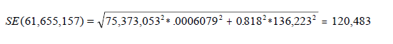
Example 5 - Calculating the Standard Error of a Product
We are interested in the number of 1-unit detached owner-occupied housing units. The number of owner-occupied housing units is 75,373,053 with a margin of error of 224,087 from subject table S2504 for 2008, and the percent of 1-unit detached owner-occupied housing units is 81.8% (0.818) with a margin of error of 0.1 (0.001). So the number of 1- unit detached owner-occupied housing units is 75,373,053 * 0.818 = 61,655,157. Calculating the standard error for the estimates using the margin of error we have:
SE(75,373,053) = 224,087 / 1.645 = 136,223 and SE(0.818) = 0.001 / 1.645 = 0.0006079
The standard error for number of 1-unit detached owner-occupied housing units is calculated using the formula for products as:
To calculate the lower and upper bounds of the 90 percent confidence interval around 61,655,157 using the standard error, simply multiply 120,483 by 1.645, then add and subtract the product from 61,655,157. Thus the 90 percent confidence interval for this estimate is [61,655,157 - 1.645(120,483)] to [61,655,157 + 1.645(120,483)] or 61,456,962 to 61,853,352.
As mentioned earlier, sample data are subject to nonsampling error. This component of error could introduce serious bias into the data, and the total error could increase dramatically over that which would result purely from sampling. While it is impossible to completely eliminate nonsampling error from a survey operation, the Census Bureau attempts to control the sources of such error during the collection and processing operations. Described below are the primary sources of nonsampling error and the programs instituted for control of this error. The success of these programs, however, is contingent upon how well the instructions were carried out during the survey.
A major way to avoid coverage error in a survey is to ensure that its sampling frame, for ACS an address list in each state, is as complete and accurate as possible. The source of addresses for the ACS is the MAF, which was created by combining the Delivery Sequence File of the United States Postal Service and the address list for Census 2000. An attempt is made to assign all appropriate geographic codes to each MAF address via an automated procedure using the Census Bureau TIGER (Topologically Integrated Geographic Encoding and Referencing) files. A manual coding operation based in the appropriate regional offices is attempted for addresses, which could not be automatically coded. The MAF was used as the source of addresses for selecting sample housing units and mailing questionnaires. TIGER produced the location maps for CAPI assignments. Sometimes the MAF has an address that is the duplicate of another address already on the MAF. This could occur when there is a slight difference in the address such as 123 Main Street versus 123 Maine Street.
In the CATI and CAPI nonresponse follow-up phases, efforts were made to minimize the chances that housing units that were not part of the sample were interviewed in place of units in sample by mistake. If a CATI interviewer called a mail nonresponse case and was not able to reach the exact address, no interview was conducted and the case was eligible for CAPI. During CAPI follow-up, the interviewer had to locate the exact address for each sample housing unit. If the interviewer could not locate the exact sample unit in a multi-unit structure, or found a different number of units than expected, the interviewers were instructed to list the units in the building and follow a specific procedure to select a replacement sample unit. Person overcoverage can occur when an individual is included as a member of a housing unit but does not meet ACS residency rules.
Coverage rates give a measure of undercoverage or overcoverage of persons or housing units in a given geographic area. Rates below 100 percent indicate undercoverage, while rates above 100 percent indicate overcoverage. Coverage rates are released concurrent with the release of estimates on American FactFinder in the B98 series of detailed tables. Further information about ACS coverage rates may be found at http://www.census.gov/acs/www/UseData/sse/cov/cov_def.htm
The ACS made every effort to minimize unit nonresponse, and thus, the potential for nonresponse error. First, the ACS used a combination of mail, CATI, and CAPI data collection modes to maximize response. The mail phase included a series of three to four mailings to encourage housing units to return the questionnaire. Subsequently, mail nonrespondents (for which phone numbers are available) were contacted by CATI for an interview. Finally, a subsample of the mail and telephone nonrespondents was contacted for by personal visit to attempt an interview. Combined, these three efforts resulted in a very high overall response rate for the ACS.
ACS response rates measure the percent of units with a completed interview. The higher the response rate, and consequently the lower the nonresponse rate, the less chance estimates may be affected by nonresponse bias. Response and nonresponse rates, as well as rates for specific types of nonresponse, are released concurrent with the release of estimates on American FactFinder in the B98 series of detailed tables. Further information about response and nonresponse rates may be found at http://www.census.gov/acs/www/UseData/sse/cov/cov_def.htm
Some protection against the introduction of large errors or biases is afforded by minimizing nonresponse. In the ACS, item nonresponse for the CATI and CAPI operations was minimized by the requirement that the automated instrument receive a response to each question before the next one could be asked. Questionnaires returned by mail were edited for completeness and acceptability. They were reviewed by computer for content omissions and population coverage. If necessary, a telephone follow-up was made to obtain missing information. Potential coverage errors were included in this follow-up.
Allocation tables provide the weighted estimate of persons or housing units for which a value was imputed, as well as the total estimate of persons or housing units that were eligible to answer the question. The smaller the number of imputed responses, the lower the chance that the item nonresponse is contributing a bias to the estimates. Allocation tables are released concurrent with the release of estimates on American Factfinder in the B99 series of detailed tables with the overall allocation rates across all person and housing unit characteristics in the B98 series of detailed tables. Additional information on item nonresponse and allocations can be found at http://www.census.gov/acs/www/UseData/sse/cov/cov_def.htm
- Coverage Error
A major way to avoid coverage error in a survey is to ensure that its sampling frame, for ACS an address list in each state, is as complete and accurate as possible. The source of addresses for the ACS is the MAF, which was created by combining the Delivery Sequence File of the United States Postal Service and the address list for Census 2000. An attempt is made to assign all appropriate geographic codes to each MAF address via an automated procedure using the Census Bureau TIGER (Topologically Integrated Geographic Encoding and Referencing) files. A manual coding operation based in the appropriate regional offices is attempted for addresses, which could not be automatically coded. The MAF was used as the source of addresses for selecting sample housing units and mailing questionnaires. TIGER produced the location maps for CAPI assignments. Sometimes the MAF has an address that is the duplicate of another address already on the MAF. This could occur when there is a slight difference in the address such as 123 Main Street versus 123 Maine Street.
In the CATI and CAPI nonresponse follow-up phases, efforts were made to minimize the chances that housing units that were not part of the sample were interviewed in place of units in sample by mistake. If a CATI interviewer called a mail nonresponse case and was not able to reach the exact address, no interview was conducted and the case was eligible for CAPI. During CAPI follow-up, the interviewer had to locate the exact address for each sample housing unit. If the interviewer could not locate the exact sample unit in a multi-unit structure, or found a different number of units than expected, the interviewers were instructed to list the units in the building and follow a specific procedure to select a replacement sample unit. Person overcoverage can occur when an individual is included as a member of a housing unit but does not meet ACS residency rules.
Coverage rates give a measure of undercoverage or overcoverage of persons or housing units in a given geographic area. Rates below 100 percent indicate undercoverage, while rates above 100 percent indicate overcoverage. Coverage rates are released concurrent with the release of estimates on American FactFinder in the B98 series of detailed tables. Further information about ACS coverage rates may be found at http://www.census.gov/acs/www/UseData/sse/cov/cov_def.htm
- Nonresponse Error
- Unit Nonresponse
The ACS made every effort to minimize unit nonresponse, and thus, the potential for nonresponse error. First, the ACS used a combination of mail, CATI, and CAPI data collection modes to maximize response. The mail phase included a series of three to four mailings to encourage housing units to return the questionnaire. Subsequently, mail nonrespondents (for which phone numbers are available) were contacted by CATI for an interview. Finally, a subsample of the mail and telephone nonrespondents was contacted for by personal visit to attempt an interview. Combined, these three efforts resulted in a very high overall response rate for the ACS.
ACS response rates measure the percent of units with a completed interview. The higher the response rate, and consequently the lower the nonresponse rate, the less chance estimates may be affected by nonresponse bias. Response and nonresponse rates, as well as rates for specific types of nonresponse, are released concurrent with the release of estimates on American FactFinder in the B98 series of detailed tables. Further information about response and nonresponse rates may be found at http://www.census.gov/acs/www/UseData/sse/cov/cov_def.htm
- Item Nonresponse
Some protection against the introduction of large errors or biases is afforded by minimizing nonresponse. In the ACS, item nonresponse for the CATI and CAPI operations was minimized by the requirement that the automated instrument receive a response to each question before the next one could be asked. Questionnaires returned by mail were edited for completeness and acceptability. They were reviewed by computer for content omissions and population coverage. If necessary, a telephone follow-up was made to obtain missing information. Potential coverage errors were included in this follow-up.
Allocation tables provide the weighted estimate of persons or housing units for which a value was imputed, as well as the total estimate of persons or housing units that were eligible to answer the question. The smaller the number of imputed responses, the lower the chance that the item nonresponse is contributing a bias to the estimates. Allocation tables are released concurrent with the release of estimates on American Factfinder in the B99 series of detailed tables with the overall allocation rates across all person and housing unit characteristics in the B98 series of detailed tables. Additional information on item nonresponse and allocations can be found at http://www.census.gov/acs/www/UseData/sse/cov/cov_def.htm
- Measurement and Processing Error
- Interviewer monitoring
- Processing Error
- Content Editing
Revised January 25, 2010
The data contained in these data products are based on the Puerto Rico Community Survey (PRCS) sample interviewed from January 1, 2008 through December 31, 2008. The PRCS sample is selected from all municipios in Puerto Rico (PR). Data for Puerto Rico was first collected in 2005 for housing units. In 2006, the PRCS began collection of data from sampled persons in group quarters (GQs) - for example, military barracks, college dormitories, nursing homes, and correctional facilities. Persons in group quarters are included with persons in housing units (HUs) in all 2008 PRCS estimates that are based on the total population. All PRCS population estimates from years prior to 2006 include only persons in housing units. The PRCS, like any other statistical activity, is subject to error. The purpose of this documentation is to provide data users with a basic understanding of the PRCS sample design, estimation methodology, and accuracy of the PRCS data. The PRCS is sponsored by the U.S. Census Bureau, and is part of the 2010 Decennial Census Program.
Additional information on the operational aspects of the PRCS, including data collection and processing, can be found in the Design and Methodology: ACS Report.
Additional information on the operational aspects of the PRCS, including data collection and processing, can be found in the Design and Methodology: ACS Report.
The PRCS employs three modes of data collection:
The general timing of data collection is:
Month 1: Addresses in sample that are determined to be mailable are sent a questionnaire via the U.S. Postal Service.
Month 2: All mail non-responding addresses with an available phone number are sent to CATI.
Month 3: A sample of mail non-responses without a phone number, CATI non-responses, and unmailable addresses are selected and sent to CAPI.
Note that mail responses are accepted during all three months of data collection.
- Mailout/Mailback
- Computer Assisted Telephone Interview (CATI)
- Computer Assisted Personal Interview (CAPI)
The general timing of data collection is:
Month 1: Addresses in sample that are determined to be mailable are sent a questionnaire via the U.S. Postal Service.
Month 2: All mail non-responding addresses with an available phone number are sent to CATI.
Month 3: A sample of mail non-responses without a phone number, CATI non-responses, and unmailable addresses are selected and sent to CAPI.
Note that mail responses are accepted during all three months of data collection.
Field representatives have several options available to them for data collection. These include completing the questionnaire while speaking to the resident in person or over the telephone, conducting a personal interview with a proxy, such as a relative or guardian, or leaving paper questionnaires for residents to complete for themselves and then pick them up later. This last option is used for data collection in Federal prisons.
Group Quarters data collection spans six weeks, except for Federal prisons, where the data collection time period is four months. All Federal prisons are assigned to September with a four month data collection window.
Group Quarters data collection spans six weeks, except for Federal prisons, where the data collection time period is four months. All Federal prisons are assigned to September with a four month data collection window.
The universe for the PRCS consists of all valid, residential housing unit addresses in all municipios in Puerto Rico. The Master Address File (MAF) is a database maintained by the Census Bureau containing a listing of residential and commercial addresses in the U.S. and Puerto Rico. The MAF is updated twice each year with the Delivery Sequence Files provided by the U.S. Postal Service, however this update covers only the U.S. The DSF does not provide changes and updates to the MAF for Puerto Rico. The MAF is also updated with the results from various Census Bureau field operations, including the PRCS.
The group quarters (GQ) sampling frame is created from the Special Place (SP)/GQ facility files, obtained from decennial census operations, merged with the MAF. This frame includes GQs added from operations such as the GQ Incomplete Information Operation (IIO) at the Census Bureau's National Processing Center in Jeffersonville, Indiana, the Census Questionnaire Resolution (CQR) Program and GQs closed on Census day. The GQ frame also underwent an unduplication process. GQs that were closed on Census day were not included in the SP/GQ inventory file received from Decennial Systems and Contract Management Office (DSCMO). These were added from a preliminary inventory file obtained from DSCMO since it was possible that while these GQs were closed on Census day, they could be open when the PRCS contacts them. Headquarters Staff researched state prisons on the Internet to obtain the current operating status and the current population counts for state prisons. After the frame was put together from these different sources, it was then sorted geographically.
The PRCS employs a two-phase, two-stage sample design. The PRCS first-phase sample consists of two separate samples, Main and Supplemental, each chosen at different points in time. Together, these constitute the first-phase sample. Both the Main and the Supplemental samples are chosen in two stages referred to as first- and second-stage sampling. Subsequent to second-stage sampling, sample addresses are randomly assigned to one of the twelve months of the sample year. The second-phase of sampling occurs when the CAPI sample is selected (see Section 2 below).
The Main sample is selected during the summer preceding the sample year. Approximately 99 percent of the sample is selected at this time. Each address in sample is randomly assigned to one of the 12 months of the sample year. Supplemental sampling occurs in January/February of the sample year and accounts for approximately 1 percent of the overall first-phase sample. The Supplemental sample is allocated to the last nine months of the sample year. A sub-sample of non-responding addresses and of any addresses deemed unmailable is selected for the CAPI data collection mode.
Several of the steps used to select the first-phase sample are common to both Main and Supplemental sampling. The descriptions of the steps included in the first-phase sample selection below indicate which are common to both and which are unique to either Main or Supplemental sampling.
1. First-phase Sample Selection
The measure of size is an estimate of the number of occupied HUs in the Municipio. This is calculated by multiplying the number of PRCS addresses by the occupancy rate from Census 2000 at the block level. A measure of size for each Census Tract is also calculated in the same manner.
Each block is then assigned the smallest measure of size from the set of all entities of which it is a part. The second-stage sampling strata and the overall first-phase sampling rates are shown in Table 1 below.
The Main sample is selected during the summer preceding the sample year. Approximately 99 percent of the sample is selected at this time. Each address in sample is randomly assigned to one of the 12 months of the sample year. Supplemental sampling occurs in January/February of the sample year and accounts for approximately 1 percent of the overall first-phase sample. The Supplemental sample is allocated to the last nine months of the sample year. A sub-sample of non-responding addresses and of any addresses deemed unmailable is selected for the CAPI data collection mode.
Several of the steps used to select the first-phase sample are common to both Main and Supplemental sampling. The descriptions of the steps included in the first-phase sample selection below indicate which are common to both and which are unique to either Main or Supplemental sampling.
1. First-phase Sample Selection
- First-stage sampling (performed during both Main and Supplemental sampling)
- Assignment of blocks to a second-stage sampling stratum (performed during Main sampling only)
The measure of size is an estimate of the number of occupied HUs in the Municipio. This is calculated by multiplying the number of PRCS addresses by the occupancy rate from Census 2000 at the block level. A measure of size for each Census Tract is also calculated in the same manner.
Each block is then assigned the smallest measure of size from the set of all entities of which it is a part. The second-stage sampling strata and the overall first-phase sampling rates are shown in Table 1 below.
- Calculation of the second-stage sampling rates (performed during Main sampling only)
- Second-stage sample selection (performed in Main and Supplemental)
- Sample Month Assignment (performed in Main and Supplemental)
| Sampling Rate Category | Sampling Rates |
|---|---|
| Blocks in smallest Municipios (MOS1 < 200) | 10.0% |
| Blocks in smaller Municipios (200 ≤ MOS < 800) | 8.04% |
| Blocks in small Municipios (800 ≤ MOS ≤ 1200) | 4.02% |
| Blocks in large Municipios (MOS >1200, TRACTMOS2≥ 2000) | 2.01% |
| All other blocks (MOS >1200, TRACTMOS < 2000) | 2.68% |
1MOS = Measure of size.
2TRACTMOS = Census Tract measure of size.
2. Second-phase Sample Selection - Subsampling the Unmailable and Non-Responding Addresses All addresses determined to be unmailable are subsampled for the CAPI phase of data collection at a rate of 2-in-3. Unmailable addresses do not go to the CATI phase of data collection. Subsequent to CATI, all addresses for which no response has been obtained prior to CAPI are subsampled based on the expected rate of completed interviews at the tract level using the rates shown in Table 2.
Table 2. Second-Phase (CAPI) Subsampling Rates for Puerto Rico
Systematic errors which are consistent in one direction introduce bias into the results of a sample survey. The Census Bureau protects against the effect of systematic errors on survey estimates by conducting extensive research and evaluation programs on sampling techniques, questionnaire design, and data collection and processing procedures. In addition, an important goal of the PRCS is to minimize the amount of nonsampling error introduced through nonresponse for sample housing units. One way of accomplishing this is by following up on mail nonrespondents during the CATI and CAPI phases.
Calculating the Standard Error from the Margin of Error
The estimated number of males, never married is 634,711 from summary table B12001 for Puerto Rico for 2008. The margin of error is 11,399.
Standard Error = Margin of Error / 1.645
Calculating the standard error using the margin of error, we have:
SE(634,711) = 11,399/ 1.645 = 6,929.
We are interested in the number of people who have never been married. From Example 1, we know the number of males, never married is 634,711. From summary table B12001 we have the number of females, never married is 576,668 with a margin of error of 10,298. So, the estimated number of people who have never been married is 634,711 + 576,668 = 1,211,379. To calculate the standard error of this sum, we need the standard errors of the two estimates in the sum. We have the standard error for the number of males never married from Example 1 as 6,929. The standard error for the number of females never married is calculated using the margin of error:
SE(576,668) = 10,298 / 1.645 = 6,260.
So using the formula for the standard error of a sum or difference we have:
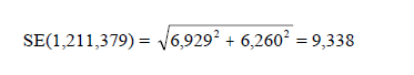
Caution: This method, however, will underestimate (overestimate) the standard error if the two items in a sum are highly positively (negatively) correlated or if the two items in a difference are highly negatively (positively) correlated.
To calculate the lower and upper bounds of the 90 percent confidence interval around 1,211,379 using the standard error, simply multiply 9,338 by 1.645, then add and subtract the product from 1,211,379. Thus the 90 percent confidence interval for this estimate is [1,211,379 - 1.645(9,338)] to [1,211,379 + 1.645(9,338)] or 1,196,018 to 1,226,740.
We are interested in the percentage of females who have never been married to the number of people who have never been married. The number of females, never married is 576,668 and the number of people who have never been married is 1,211,379. To calculate the standard error of this proportion or percent, we need the standard errors of the two estimates in the proportion. We have the standard error for the number of females never married from Example 2 as 6,260 and the standard error for the number of people never married calculated from example 2 as 9,338.
The estimate is (576,668 / 1,211,379) * 100% = 47.6%
So, using the formula for the standard error of a proportion or percent, we have:
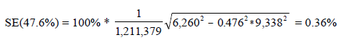
To calculate the lower and upper bounds of the 90 percent confidence interval around 47.6 using the standard error, simply multiply 0.36 by 1.645, then add and subtract the product from 47.6. Thus the 90 percent confidence interval for this estimate is [47.6 - 1.645(0.36)] to [47.6 + 1.645(0.36)], or 47.0% to 48.2%.
Now, let us calculate the estimate of the ratio of the number of unmarried males to the number of unmarried females and its standard error. From the above examples, the estimate for the number of unmarried men is 634,711 with a standard error of 6,929, and the estimate for the number of unmarried women is 576,668 with a standard error of 6,260.
The estimate of the ratio is 634,711 / 576,668 = 1.101.

The 90 percent margin of error for this estimate would be 0.017 multiplied by 1.645, or about 0.028. The 90 percent lower and upper 90 percent confidence bounds would then be [1.101- 0.028] to [1.101 + 0.028], or 1.073 and 1.129.
We are interested in the number of 1-unit detached owner-occupied housing units. The number of owner-occupied housing units is 859,531 with a margin of error of 9,334 from subject table S2504 for 2008, and the percent of 1-unit detached owner-occupied housing units is 79.7% (0.797) with a margin of error of 0.5 (0.005). So the number of 1-unit detached owner-occupied housing units is 859,531 * 0.797 = 685,046. Calculating the standard error for the estimates using the margin of error we have:
SE(859,531) = 9,334 / 1.645 = 5,674
and
SE(0.797) = 0.005 / 1.645 = 0.0030395
The standard error for number of 1-unit detached owner-occupied housing units is calculated using the formula for products as:
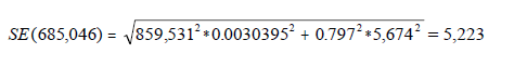
To calculate the lower and upper bounds of the 90 percent confidence interval around 685,046 using the standard error, simply multiply 5,223 by 1.645, then add and subtract the product from 685,046. Thus the 90 percent confidence interval for this estimate is [685,046 - 1.645(5,223)] to [685,046 + 1.645(5,223)] or 676,454 to 693,638.


 News Feed |
About Us |
Contact Us |
FAQ |
Terms of Use |
Privacy Policy
News Feed |
About Us |
Contact Us |
FAQ |
Terms of Use |
Privacy Policy
2TRACTMOS = Census Tract measure of size.
2. Second-phase Sample Selection - Subsampling the Unmailable and Non-Responding Addresses All addresses determined to be unmailable are subsampled for the CAPI phase of data collection at a rate of 2-in-3. Unmailable addresses do not go to the CATI phase of data collection. Subsequent to CATI, all addresses for which no response has been obtained prior to CAPI are subsampled based on the expected rate of completed interviews at the tract level using the rates shown in Table 2.
Table 2. Second-Phase (CAPI) Subsampling Rates for Puerto Rico
| Address Characteristics | CAPI Subsampling Rate | |
|---|---|---|
| Unmailable addresses | 66.7% | |
| Mailable addresses | 50% |
| Major GQ Type Group | Definition | Institutional / Non-Institutional |
|---|---|---|
| 1 | Correctional Institutions | Institutional |
| 2 | Juvenile Detention Facilities | Institutional |
| 3 | Nursing Homes | Institutional |
| 4 | Other Long-Term Care Facilities | Institutional |
| 5 | College Dormitories | Non-Institutional |
| 6 | Military Facilities | Non-Institutional |
| 7 | Other Non-Institutional Facilities | Non-Institutional |
The procedure used to assign the weights to the GQ persons is performed independently within the commonwealth of Puerto Rico. The steps to assign the weights to the GQ persons are as follows:
- Base Weight
- Non-Interview Factor
Major GQ x Type Group x Municipio
- GQ Person Post-stratification Factor
Major GQ x Type Group
- Rounding
Major GQ x Type Group
Major GQ x Type Group x Municipio
The housing unit and household person weighting use weighting areas built from collections of whole municipios. Census 2000 data are used to group municipios of similar demographic and social characteristics. The characteristics considered in the formation include:
Each weighting area is also required to meet a threshold of 400 expected person interviews in the 2008 PRCS. The process also tries to preserve as many municipios that met the threshold to form their own weighting areas. In total, there are 55 weighting areas formed from the 78 municipios in Puerto Rico.
The estimation procedure used to assign the weights is then performed independently within each of the PRCS weighting areas.
1. Initial Housing Unit Weighting Factors - This process produces the following factors:
Selected in CAPI subsampling: SSF = 2.0
Not selected in CAPI subsampling: SSF = 0.0
Not a CAPI case: SSF = 1.0
Some sample addresses are unmailable. A two-thirds sample of these is sent directly to CAPI and for these cases SSF = 1.5.
Weighting Area x Month
Weighting Area x Building Type x Tract
A second factor, NIF2, is a ratio adjustment that is computed and assigned to occupied housing units based on the following groups:
Weighting Area x Building Type x Month
NIF is then computed by applying NIF1 and NIF2 for each occupied housing unit.
Vacant housing units are assigned a value of NIF = 1.0. Nonresponding housing units are now assigned a weight of 0.0.
NIFM is computed and assigned to occupied CAPI housing units based on the following groups:
Weighting Area x Building Type (single or multi unit) x Month
Vacant housing units or non-CAPI (mail and CATI) housing units receive a value of NIFM = 1.0.
Weighting Area x Tenure (owner or renter) x Month x Marital Status of the Householder (married/widowed or single)
Vacant housing units receive a value of MBF = 1.0. MBF is applied to the weights computed through NIF.
2. Person Weighting Factors - Initially the person weight of each person in an occupied housing unit is the product of the weighting factors of their associated housing unit (BW x ... x MBF). At this point everyone in the household has the same weight. Beginning in 2006, the person weighting is done in a series of three steps which are repeated until a stopping criterion is met. These three steps form a raking ratio or raking process. These person weights are individually adjusted for each person as described below.
The three steps are as follows:
- Householder in a married-couple or unmarried-partner household
- Spouse or unmarried partner in a married-couple or unmarried-partner household
- All others
The first two groups are adjusted so that the sum of their person weights is equal to the total estimate of married-couple or unmarried-partner households using the housing unit weight (BW x ... x MBF). The goal of this step is to produce more consistent estimates of spouses or unmarried partners and married-couple and unmarried-partner households.
- Householders
- Non-householders
The first group is adjusted so that the sum of their person weights is equal to the total estimate of occupied housing units using the housing unit weight (BW x ... x MBF). The goal of this step is to produce more consistent estimates of householders, occupied housing units, and households.
Demographic Raking Factor (DEMORF) - This factor is applied to individuals based on their age and sex in Puerto Rico (note that there are 13 Age groupings). It adjusts the person weights so that the weighted sample counts equal the independent population estimates by age and sex at the weighting area level. Because of collapsing of groups in applying this factor, only the total population is assured of agreeing with the official 2008 population estimates at the weighting area level.
These three steps are repeated several times until the estimates for Puerto Rico achieve their optimal consistency with regard to the spouse and householder equalization. The Person Post-Stratification Factor (PPSF) is then equal to the product (SPEQRF x HHEQRF x DEMORF) from all of iterations of these three adjustments. The unrounded person weight is then the equal to the product of PPSF times the housing unit weight (BW x ... x MBF x PPSF).
3. Rounding - The final product of all person weights (BW x ... x MBF x PPSF) is rounded to an integer. Rounding is performed so that the sum of the rounded weights is within one person of the sum of the unrounded weights for any of the groups listed below:
Municipio
Municipio x Sex
Municipio x Sex x Age
Municipio x Sex x Age x Tract
Municipio x Sex x Age x Tract x Block
For example, the number of White, Males, Age 30 estimated for a municipio using the rounded weights is within one of the number produced using the unrounded weights.
4. Final Housing Unit Weighting Factors - This process produces the following factors:
Municipio
Municipio x Tract
Municipio x Tract x Block
- Percent in poverty
- Percent renting
- Percent in rural areas
- Race/ethnicity, age, and sex distribution
- Distance between the centroids of the municipios
- Core-based Statistical Area status
Each weighting area is also required to meet a threshold of 400 expected person interviews in the 2008 PRCS. The process also tries to preserve as many municipios that met the threshold to form their own weighting areas. In total, there are 55 weighting areas formed from the 78 municipios in Puerto Rico.
The estimation procedure used to assign the weights is then performed independently within each of the PRCS weighting areas.
1. Initial Housing Unit Weighting Factors - This process produces the following factors:
- Base Weight (BW)
- CAPI Subsampling Factor (SSF)
Selected in CAPI subsampling: SSF = 2.0
Not selected in CAPI subsampling: SSF = 0.0
Not a CAPI case: SSF = 1.0
Some sample addresses are unmailable. A two-thirds sample of these is sent directly to CAPI and for these cases SSF = 1.5.
- Variation in Monthly Response by Mode (VMS)
Weighting Area x Month
- Noninterview Factor (NIF)
Weighting Area x Building Type x Tract
A second factor, NIF2, is a ratio adjustment that is computed and assigned to occupied housing units based on the following groups:
Weighting Area x Building Type x Month
NIF is then computed by applying NIF1 and NIF2 for each occupied housing unit.
Vacant housing units are assigned a value of NIF = 1.0. Nonresponding housing units are now assigned a weight of 0.0.
- Noninterview Factor - Mode (NIFM)
NIFM is computed and assigned to occupied CAPI housing units based on the following groups:
Weighting Area x Building Type (single or multi unit) x Month
Vacant housing units or non-CAPI (mail and CATI) housing units receive a value of NIFM = 1.0.
- Mode Bias Factor (MBF)
Weighting Area x Tenure (owner or renter) x Month x Marital Status of the Householder (married/widowed or single)
Vacant housing units receive a value of MBF = 1.0. MBF is applied to the weights computed through NIF.
2. Person Weighting Factors - Initially the person weight of each person in an occupied housing unit is the product of the weighting factors of their associated housing unit (BW x ... x MBF). At this point everyone in the household has the same weight. Beginning in 2006, the person weighting is done in a series of three steps which are repeated until a stopping criterion is met. These three steps form a raking ratio or raking process. These person weights are individually adjusted for each person as described below.
The three steps are as follows:
- Spouse Equalization Raking Factor (SPEQRF)
- Householder in a married-couple or unmarried-partner household
- Spouse or unmarried partner in a married-couple or unmarried-partner household
- All others
The first two groups are adjusted so that the sum of their person weights is equal to the total estimate of married-couple or unmarried-partner households using the housing unit weight (BW x ... x MBF). The goal of this step is to produce more consistent estimates of spouses or unmarried partners and married-couple and unmarried-partner households.
- Householder Equalization Raking Factor (HHEQRF)
- Householders
- Non-householders
The first group is adjusted so that the sum of their person weights is equal to the total estimate of occupied housing units using the housing unit weight (BW x ... x MBF). The goal of this step is to produce more consistent estimates of householders, occupied housing units, and households.
Demographic Raking Factor (DEMORF) - This factor is applied to individuals based on their age and sex in Puerto Rico (note that there are 13 Age groupings). It adjusts the person weights so that the weighted sample counts equal the independent population estimates by age and sex at the weighting area level. Because of collapsing of groups in applying this factor, only the total population is assured of agreeing with the official 2008 population estimates at the weighting area level.
These three steps are repeated several times until the estimates for Puerto Rico achieve their optimal consistency with regard to the spouse and householder equalization. The Person Post-Stratification Factor (PPSF) is then equal to the product (SPEQRF x HHEQRF x DEMORF) from all of iterations of these three adjustments. The unrounded person weight is then the equal to the product of PPSF times the housing unit weight (BW x ... x MBF x PPSF).
3. Rounding - The final product of all person weights (BW x ... x MBF x PPSF) is rounded to an integer. Rounding is performed so that the sum of the rounded weights is within one person of the sum of the unrounded weights for any of the groups listed below:
Municipio
Municipio x Sex
Municipio x Sex x Age
Municipio x Sex x Age x Tract
Municipio x Sex x Age x Tract x Block
For example, the number of White, Males, Age 30 estimated for a municipio using the rounded weights is within one of the number produced using the unrounded weights.
4. Final Housing Unit Weighting Factors - This process produces the following factors:
- Householder Factor (HHF)
- Rounding
Municipio
Municipio x Tract
Municipio x Tract x Block
The Census Bureau has modified or suppressed some data on this site to protect confidentiality. Title 13 United States Code, Section 9, prohibits the Census Bureau from publishing results in which an individual's data can be identified.
The Census Bureau's internal Disclosure Review Board sets the confidentiality rules for all data releases. A checklist approach is used to ensure that all potential risks to the confidentiality of the data are considered and addressed.
The Census Bureau's internal Disclosure Review Board sets the confidentiality rules for all data releases. A checklist approach is used to ensure that all potential risks to the confidentiality of the data are considered and addressed.
- Title 13, United States Code
- Disclosure Avoidance
- Data Swapping
- Synthetic Data
- Sampling Error
- Nonsampling Error
Systematic errors which are consistent in one direction introduce bias into the results of a sample survey. The Census Bureau protects against the effect of systematic errors on survey estimates by conducting extensive research and evaluation programs on sampling techniques, questionnaire design, and data collection and processing procedures. In addition, an important goal of the PRCS is to minimize the amount of nonsampling error introduced through nonresponse for sample housing units. One way of accomplishing this is by following up on mail nonrespondents during the CATI and CAPI phases.
Sampling error is the difference between an estimate based on a sample and the corresponding value that would be obtained if the estimate were based on the entire population (as from a census). Note that sample-based estimates will vary depending on the particular sample selected from the population. Measures of the magnitude of sampling error reflect the variation in the estimates over all possible samples that could have been selected from the population using the same sampling methodology.
Estimates of the magnitude of sampling errors - in the form of margins of error - are provided with all published PRCS data. The Census Bureau recommends that data users incorporate this information into their analyses, as sampling error in survey estimates could impact the conclusions drawn from the results.
Estimates of the magnitude of sampling errors - in the form of margins of error - are provided with all published PRCS data. The Census Bureau recommends that data users incorporate this information into their analyses, as sampling error in survey estimates could impact the conclusions drawn from the results.
Confidence Intervals - A sample estimate and its estimated standard error may be used to construct confidence intervals about the estimate. These intervals are ranges that will contain the average value of the estimated characteristic that results over all possible samples, with a known probability.
For example, if all possible samples that could result under the PRCS sample design were independently selected and surveyed under the same conditions, and if the estimate and its estimated standard error were calculated for each of these samples, then:
1. Approximately 68 percent of the intervals from one estimated standard error below the estimate to one estimated standard error above the estimate would contain the average result from all possible samples;
2. Approximately 90 percent of the intervals from 1.645 times the estimated standard error below the estimate to 1.645 times the estimated standard error above the estimate would contain the average result from all possible samples.
3. Approximately 95 percent of the intervals from two estimated standard errors below the estimate to two estimated standard errors above the estimate would contain the average result from all possible samples.
The intervals are referred to as 68 percent, 90 percent, and 95 percent confidence intervals, respectively.
Margin of Error - Instead of providing the upper and lower confidence bounds in published PRCS tables, the margin of error is provided instead. The margin of error is the difference between an estimate and its upper or lower confidence bound. Both the confidence bounds and the standard error can easily be computed from the margin of error. All PRCS published margins of error are based on a 90 percent confidence level.
Standard Error = Margin of Error / 1.645
Lower Confidence Bound = Estimate - Margin of Error
Upper Confidence Bound = Estimate + Margin of Error
Note that for 2005, PRCS margins of error and confidence bounds were calculated using a 90 percent confidence level multiplier of 1.65. Beginning with the 2006 data release, we are now employing a more accurate multiplier of 1.645. Margins of error and confidence bounds from previously published products will not be updated with the new multiplier. When calculating standard errors from margins of error or confidence bounds using published data for 2005, use the 1.65 multiplier.
When constructing confidence bounds from the margin of error, the user should be aware of any "natural" limits on the bounds. For example, if a population estimate is near zero, the calculated value of the lower confidence bound may be negative. However, a negative number of people does not make sense, so the lower confidence bound should be reported as zero instead. However, for other estimates such as income, negative values do make sense. The context and meaning of the estimate must be kept in mind when creating these bounds. Another of these natural limits would be 100 percent for the upper bound of a percent estimate.
If the margin of error is displayed as "*****" (five asterisks), the estimate has been controlled to be equal to a fixed value and so it has no sampling error. When using any of the formulas in the following section, use a standard error of zero for these controlled estimates. Limitations -The user should be careful when computing and interpreting confidence intervals.
- The estimated standard errors (and thus margins of error) included in these data products do not include portions of the variability due to nonsampling error that may be present in the data. In particular, the standard errors do not reflect the effect of correlated errors introduced by interviewers, coders, or other field or processing personnel. Nor do they reflect the error from imputed values due to missing responses. Thus, the standard errors calculated represent a lower bound of the total error. As a result, confidence intervals formed using these estimated standard errors may not meet the stated levels of confidence (i.e., 68, 90, or 95 percent). Thus, some care must be exercised in the interpretation of the data in this data product based on the estimated standard errors.
- Zero or small estimates; very large estimates - The value of almost all PRCS characteristics is greater than or equal to zero by definition. For zero or small estimates, use of the method given previously for calculating confidence intervals relies on large sample theory, and may result in negative values which for most characteristics are not admissible. In this case the lower limit of the confidence interval is set to zero by default. A similar caution holds for estimates of totals close to control total or estimated proportions near one, where the upper limit of the confidence interval is set to its largest admissible value. In these situations the level of confidence of the adjusted range of values is less than the prescribed confidence level.
Direct estimates of the standard errors were calculated for all estimates reported in this product. The standard errors, in most cases, are calculated using a replicate-based methodology that takes into account the sample design and estimation procedures. Excluding the base weights, replicate weights were allowed to be negative in order to avoid underestimating the standard error.
Exceptions include:
1. The estimate of the number or proportion of people, households, families, or housing units in a geographic area with a specific characteristic is zero. A special procedure is used to estimate the standard error.
2. There are either no sample observations available to compute an estimate or standard error of a median, an aggregate, a proportion, or some other ratio, or there are too few sample observations to compute a stable estimate of the standard error. The estimate is represented in the tables by "-" and the margin of error by "**" (two asterisks).
3. The estimate of a median falls in the lower open-ended interval or upper open-ended interval of a distribution. If the median occurs in the lowest interval, then a "-" follows the estimate, and if the median occurs in the upper interval, then a "+" follows the estimate. In both cases the margin of error is represented in the tables by "***" (three asterisks).
Sums and Differences of Direct Standard Errors - The standard errors estimated from these tables are for individual estimates. Additional calculations are required to estimate the standard errors for sums of and differences between two sample estimates. The estimate of the standard error of a sum or difference is approximately the square root of the sum of the two individual standard errors squared; that is, for standard errors SE (Xˆ) and SE (Yˆ) of estimates Xˆ and Yˆ:

This method, however, will underestimate (overestimate) the standard error if the two items in a sum are highly positively (negatively) correlated or if the two items in a difference are highly negatively (positively) correlated.
Ratios - The statistic of interest may be the ratio of two estimates. First is the case where the numerator is not a subset of the denominator. The standard error of this ratio between two sample estimates is approximated as:
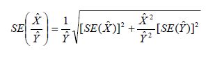
Proportions/percents - For a proportion (or percent), a ratio where the numerator is a subset of the denominator, a slightly different estimator is used. Note the difference between the formulas for the standard error for proportions (below) and ratios (above) - the plus sign in the previous formula has been replaced with a minus sign. If the value under the square root sign is negative, use the ratio standard error formula above, instead. If Pˆ = Xˆ /Yˆ , then
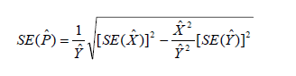
If Qˆ =100%xPˆ (P is the proportion and Q is its corresponding percent), then
SE(Qˆ ) =100% xSE(Pˆ) .
Products - For a product of two estimates - for example if you want to estimate a proportions numerator by multiplying the proportion by its denominator - the standard error can be approximated as
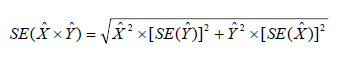
Significant differences - Users may conduct a statistical test to see if the difference between a PRCS estimate and any other chosen estimates is statistically significant at a given confidence level. "Statistically significant" means that the difference is not likely due to random chance alone. With the two estimates (Est1 and Est2) and their respective standard errors (SE1 and SE2), calculate
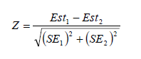
If Z > 1.645 or Z < -1.645, then the difference can be said to be statistically significant at the 90 percent confidence level. [Note that we are now recommending that +/-1.645 be used to determine significance. Previous published Accuracy of the Data documents suggested using +/- 1.65.] Any estimate can be compared to a PRCS estimate using this method, including other PRCS estimates from the current year, the PRCS estimate for the same characteristic and
geographic area but from a previous year, ACS estimates, Census 2000 100 percent counts and long form estimates, estimates from other Census Bureau surveys, and estimates from other sources. Not all estimates have sampling error - Census 2000 100 percent counts do not, for example, although Census 2000 long form estimates do - but they should be used if they exist to give the most accurate result of the test.
Users are also cautioned to not rely on looking at whether confidence intervals for two estimates overlap to determine statistical significance, because there are circumstances where that method will not give the correct test result. The Z calculation above is recommended in all cases. All statistical testing in PRCS data products is based on the 90 percent confidence level. Users should understand that all testing was done using unrounded estimates and standard errors, and it may not be possible to replicate test results using the rounded estimates and margins of error as published.
Exceptions include:
1. The estimate of the number or proportion of people, households, families, or housing units in a geographic area with a specific characteristic is zero. A special procedure is used to estimate the standard error.
2. There are either no sample observations available to compute an estimate or standard error of a median, an aggregate, a proportion, or some other ratio, or there are too few sample observations to compute a stable estimate of the standard error. The estimate is represented in the tables by "-" and the margin of error by "**" (two asterisks).
3. The estimate of a median falls in the lower open-ended interval or upper open-ended interval of a distribution. If the median occurs in the lowest interval, then a "-" follows the estimate, and if the median occurs in the upper interval, then a "+" follows the estimate. In both cases the margin of error is represented in the tables by "***" (three asterisks).
Sums and Differences of Direct Standard Errors - The standard errors estimated from these tables are for individual estimates. Additional calculations are required to estimate the standard errors for sums of and differences between two sample estimates. The estimate of the standard error of a sum or difference is approximately the square root of the sum of the two individual standard errors squared; that is, for standard errors SE (Xˆ) and SE (Yˆ) of estimates Xˆ and Yˆ:
This method, however, will underestimate (overestimate) the standard error if the two items in a sum are highly positively (negatively) correlated or if the two items in a difference are highly negatively (positively) correlated.
Ratios - The statistic of interest may be the ratio of two estimates. First is the case where the numerator is not a subset of the denominator. The standard error of this ratio between two sample estimates is approximated as:
Proportions/percents - For a proportion (or percent), a ratio where the numerator is a subset of the denominator, a slightly different estimator is used. Note the difference between the formulas for the standard error for proportions (below) and ratios (above) - the plus sign in the previous formula has been replaced with a minus sign. If the value under the square root sign is negative, use the ratio standard error formula above, instead. If Pˆ = Xˆ /Yˆ , then
If Qˆ =100%xPˆ (P is the proportion and Q is its corresponding percent), then
SE(Qˆ ) =100% xSE(Pˆ) .
Products - For a product of two estimates - for example if you want to estimate a proportions numerator by multiplying the proportion by its denominator - the standard error can be approximated as
Significant differences - Users may conduct a statistical test to see if the difference between a PRCS estimate and any other chosen estimates is statistically significant at a given confidence level. "Statistically significant" means that the difference is not likely due to random chance alone. With the two estimates (Est1 and Est2) and their respective standard errors (SE1 and SE2), calculate
If Z > 1.645 or Z < -1.645, then the difference can be said to be statistically significant at the 90 percent confidence level. [Note that we are now recommending that +/-1.645 be used to determine significance. Previous published Accuracy of the Data documents suggested using +/- 1.65.] Any estimate can be compared to a PRCS estimate using this method, including other PRCS estimates from the current year, the PRCS estimate for the same characteristic and
geographic area but from a previous year, ACS estimates, Census 2000 100 percent counts and long form estimates, estimates from other Census Bureau surveys, and estimates from other sources. Not all estimates have sampling error - Census 2000 100 percent counts do not, for example, although Census 2000 long form estimates do - but they should be used if they exist to give the most accurate result of the test.
Users are also cautioned to not rely on looking at whether confidence intervals for two estimates overlap to determine statistical significance, because there are circumstances where that method will not give the correct test result. The Z calculation above is recommended in all cases. All statistical testing in PRCS data products is based on the 90 percent confidence level. Users should understand that all testing was done using unrounded estimates and standard errors, and it may not be possible to replicate test results using the rounded estimates and margins of error as published.
- Example 1.
Calculating the Standard Error from the Margin of Error
The estimated number of males, never married is 634,711 from summary table B12001 for Puerto Rico for 2008. The margin of error is 11,399.
Standard Error = Margin of Error / 1.645
Calculating the standard error using the margin of error, we have:
SE(634,711) = 11,399/ 1.645 = 6,929.
- Example 2.
We are interested in the number of people who have never been married. From Example 1, we know the number of males, never married is 634,711. From summary table B12001 we have the number of females, never married is 576,668 with a margin of error of 10,298. So, the estimated number of people who have never been married is 634,711 + 576,668 = 1,211,379. To calculate the standard error of this sum, we need the standard errors of the two estimates in the sum. We have the standard error for the number of males never married from Example 1 as 6,929. The standard error for the number of females never married is calculated using the margin of error:
SE(576,668) = 10,298 / 1.645 = 6,260.
So using the formula for the standard error of a sum or difference we have:
Caution: This method, however, will underestimate (overestimate) the standard error if the two items in a sum are highly positively (negatively) correlated or if the two items in a difference are highly negatively (positively) correlated.
To calculate the lower and upper bounds of the 90 percent confidence interval around 1,211,379 using the standard error, simply multiply 9,338 by 1.645, then add and subtract the product from 1,211,379. Thus the 90 percent confidence interval for this estimate is [1,211,379 - 1.645(9,338)] to [1,211,379 + 1.645(9,338)] or 1,196,018 to 1,226,740.
- Example 3.
We are interested in the percentage of females who have never been married to the number of people who have never been married. The number of females, never married is 576,668 and the number of people who have never been married is 1,211,379. To calculate the standard error of this proportion or percent, we need the standard errors of the two estimates in the proportion. We have the standard error for the number of females never married from Example 2 as 6,260 and the standard error for the number of people never married calculated from example 2 as 9,338.
The estimate is (576,668 / 1,211,379) * 100% = 47.6%
So, using the formula for the standard error of a proportion or percent, we have:
To calculate the lower and upper bounds of the 90 percent confidence interval around 47.6 using the standard error, simply multiply 0.36 by 1.645, then add and subtract the product from 47.6. Thus the 90 percent confidence interval for this estimate is [47.6 - 1.645(0.36)] to [47.6 + 1.645(0.36)], or 47.0% to 48.2%.
- Example 4.
Now, let us calculate the estimate of the ratio of the number of unmarried males to the number of unmarried females and its standard error. From the above examples, the estimate for the number of unmarried men is 634,711 with a standard error of 6,929, and the estimate for the number of unmarried women is 576,668 with a standard error of 6,260.
The estimate of the ratio is 634,711 / 576,668 = 1.101.
The 90 percent margin of error for this estimate would be 0.017 multiplied by 1.645, or about 0.028. The 90 percent lower and upper 90 percent confidence bounds would then be [1.101- 0.028] to [1.101 + 0.028], or 1.073 and 1.129.
- Example 5.
We are interested in the number of 1-unit detached owner-occupied housing units. The number of owner-occupied housing units is 859,531 with a margin of error of 9,334 from subject table S2504 for 2008, and the percent of 1-unit detached owner-occupied housing units is 79.7% (0.797) with a margin of error of 0.5 (0.005). So the number of 1-unit detached owner-occupied housing units is 859,531 * 0.797 = 685,046. Calculating the standard error for the estimates using the margin of error we have:
SE(859,531) = 9,334 / 1.645 = 5,674
and
SE(0.797) = 0.005 / 1.645 = 0.0030395
The standard error for number of 1-unit detached owner-occupied housing units is calculated using the formula for products as:
To calculate the lower and upper bounds of the 90 percent confidence interval around 685,046 using the standard error, simply multiply 5,223 by 1.645, then add and subtract the product from 685,046. Thus the 90 percent confidence interval for this estimate is [685,046 - 1.645(5,223)] to [685,046 + 1.645(5,223)] or 676,454 to 693,638.
As mentioned earlier, sample data are subject to nonsampling error. This component of error could introduce serious bias into the data, and the total error could increase dramatically over that which would result purely from sampling. While it is impossible to completely eliminate nonsampling error from a survey operation, the Census Bureau attempts to control the sources of such error during the collection and processing operations. Described below are the primary sources of nonsampling error and the programs instituted for control of this error. The success of these programs, however, is contingent upon how well the instructions were carried out during the survey.
A major way to avoid coverage error in a survey is to ensure that its sampling frame, for Puerto Rico an address list in each municipio, is as complete and accurate as possible. The source of addresses for the PRCS is the MAF, which was created using the address list for Census 2000. An attempt is made to assign all appropriate geographic codes to each MAF address via an automated procedure using the Census Bureau TIGER (Topologically Integrated Geographic Encoding and Referencing) files. A manual coding operation based in the appropriate regional offices is attempted for addresses, which could not be automatically coded. The MAF was used as the source of addresses for selecting sample housing units and mailing questionnaires. TIGER produced the location maps for CAPI assignments. Sometimes the MAF has an address that is the duplicate of another address already on the MAF. This could occur when there is a slight difference in the address such as 123 Calle 1, Bayamon versus URB Hermosillo, 123 Calle 1, Bayamon.
In the CATI and CAPI nonresponse follow-up phases, efforts were made to minimize the chances that housing units that were not part of the sample were interviewed in place of units in sample by mistake. If a CATI interviewer called a mail nonresponse case and was not able to reach the exact address, no interview was conducted and the case was eligible for CAPI. During CAPI follow-up, the interviewer had to locate the exact address for each sample housing unit. If the interviewer could not locate the exact sample unit in a multi-unit structure, or found a different number of units than expected, the interviewers were instructed to list the units in the building and follow a specific procedure to select a replacement sample unit. Person overcoverage can occur when an individual is included as a member of a housing unit but does not meet PRCS residency rules.
Coverage rates give a measure of undercoverage or overcoverage of persons or housing units in a given geographic area. Rates below 100 percent indicate undercoverage, while rates above 100 percent indicate overcoverage. Coverage rates are released concurrent with the release of estimates on American FactFinder in the B98 series of detailed tables. Further information about PRCS coverage rates may be found at http://www.census.gov/acs/www/UseData/sse/cov/cov_def.htm
The PRCS made every effort to minimize unit nonresponse, and thus, the potential for nonresponse error. First, the PRCS used a combination of mail, CATI, and CAPI data collection modes to maximize response. The mail phase included a series of three to four mailings to encourage housing units to return the questionnaire. Subsequently, mail nonrespondents (for which phone numbers are available) were contacted by CATI for an interview. Finally, a subsample of the mail and telephone nonrespondents was contacted for by personal visit to attempt an interview PRCS response rates measure the percent of units with a completed interview. The higher the response rate, and consequently the lower the nonresponse rate, the less chance estimates may be affected by nonresponse bias. Response and nonresponse rates, as well as rates for specific types of nonresponse, are released concurrent with the release of estimates on American FactFinder in the B98 series of detailed tables. Further information about response and nonresponse rates may be found at http://www.census.gov/acs/www/UseData/sse/res/res_def.htm
Some protection against the introduction of large errors or biases is afforded by minimizing nonresponse. In the PRCS, item nonresponse for the CATI and CAPI operations was minimized by the requirement that the automated instrument receive a response to each question before the next one could be asked. Questionnaires returned by mail were edited for completeness and acceptability. They were reviewed by computer for content omissions and population coverage. If necessary, a telephone follow-up was made to obtain missing information. Potential coverage errors were included in this follow-up.
Allocation tables provide the weighted estimate of persons or housing units for which a value was imputed, as well as the total estimate of persons or housing units that were eligible to answer the question. The smaller the number of imputed responses, the lower the chance that the item nonresponse is contributing a bias to the estimates. Allocation tables are released concurrent with the release of estimates on American Factfinder in the B99 series of detailed tables with the overall allocation rates across all person and housing unit characteristics in the B98 series of detailed tables. Additional information on item nonresponse and allocations can be found at
http://www.census.gov/acs/www/UseData/sse/ita/ita_def.htm
- Coverage Error
A major way to avoid coverage error in a survey is to ensure that its sampling frame, for Puerto Rico an address list in each municipio, is as complete and accurate as possible. The source of addresses for the PRCS is the MAF, which was created using the address list for Census 2000. An attempt is made to assign all appropriate geographic codes to each MAF address via an automated procedure using the Census Bureau TIGER (Topologically Integrated Geographic Encoding and Referencing) files. A manual coding operation based in the appropriate regional offices is attempted for addresses, which could not be automatically coded. The MAF was used as the source of addresses for selecting sample housing units and mailing questionnaires. TIGER produced the location maps for CAPI assignments. Sometimes the MAF has an address that is the duplicate of another address already on the MAF. This could occur when there is a slight difference in the address such as 123 Calle 1, Bayamon versus URB Hermosillo, 123 Calle 1, Bayamon.
In the CATI and CAPI nonresponse follow-up phases, efforts were made to minimize the chances that housing units that were not part of the sample were interviewed in place of units in sample by mistake. If a CATI interviewer called a mail nonresponse case and was not able to reach the exact address, no interview was conducted and the case was eligible for CAPI. During CAPI follow-up, the interviewer had to locate the exact address for each sample housing unit. If the interviewer could not locate the exact sample unit in a multi-unit structure, or found a different number of units than expected, the interviewers were instructed to list the units in the building and follow a specific procedure to select a replacement sample unit. Person overcoverage can occur when an individual is included as a member of a housing unit but does not meet PRCS residency rules.
Coverage rates give a measure of undercoverage or overcoverage of persons or housing units in a given geographic area. Rates below 100 percent indicate undercoverage, while rates above 100 percent indicate overcoverage. Coverage rates are released concurrent with the release of estimates on American FactFinder in the B98 series of detailed tables. Further information about PRCS coverage rates may be found at http://www.census.gov/acs/www/UseData/sse/cov/cov_def.htm
- Nonresponse Error
- Unit Nonresponse
The PRCS made every effort to minimize unit nonresponse, and thus, the potential for nonresponse error. First, the PRCS used a combination of mail, CATI, and CAPI data collection modes to maximize response. The mail phase included a series of three to four mailings to encourage housing units to return the questionnaire. Subsequently, mail nonrespondents (for which phone numbers are available) were contacted by CATI for an interview. Finally, a subsample of the mail and telephone nonrespondents was contacted for by personal visit to attempt an interview PRCS response rates measure the percent of units with a completed interview. The higher the response rate, and consequently the lower the nonresponse rate, the less chance estimates may be affected by nonresponse bias. Response and nonresponse rates, as well as rates for specific types of nonresponse, are released concurrent with the release of estimates on American FactFinder in the B98 series of detailed tables. Further information about response and nonresponse rates may be found at http://www.census.gov/acs/www/UseData/sse/res/res_def.htm
- Item Nonresponse
Some protection against the introduction of large errors or biases is afforded by minimizing nonresponse. In the PRCS, item nonresponse for the CATI and CAPI operations was minimized by the requirement that the automated instrument receive a response to each question before the next one could be asked. Questionnaires returned by mail were edited for completeness and acceptability. They were reviewed by computer for content omissions and population coverage. If necessary, a telephone follow-up was made to obtain missing information. Potential coverage errors were included in this follow-up.
Allocation tables provide the weighted estimate of persons or housing units for which a value was imputed, as well as the total estimate of persons or housing units that were eligible to answer the question. The smaller the number of imputed responses, the lower the chance that the item nonresponse is contributing a bias to the estimates. Allocation tables are released concurrent with the release of estimates on American Factfinder in the B99 series of detailed tables with the overall allocation rates across all person and housing unit characteristics in the B98 series of detailed tables. Additional information on item nonresponse and allocations can be found at
http://www.census.gov/acs/www/UseData/sse/ita/ita_def.htm
- Measurement and Processing Error
- Interviewer monitoring
- Processing Error
- Content Editing
©2024 Social Explorer. All rights reserved.