


| Documentation: | ACS 2009 (3-Year Estimates) |
you are here:
choose a survey
survey
document
chapter
Publisher: U.S. Census Bureau
Survey: ACS 2009 (3-Year Estimates)
| Document: | ACS 2009-3yr Summary File: Technical Documentation |
| citation: | Social Explorer; U.S. Census Bureau; American Community Survey 2007-2009 Summary File: Technical Documentation. |
Chapter Contents
There are two methods to easily find the 2005-2009 ACS 5-year Summary File: (1) through the ACS home page at www.census.gov/acs or (2) through the American FactFinder web site at factfinder.census.gov.

That will take you to the ACS Summary File page. As you can see at the top of the next page, the data are arranged by each ACS data year and estimate type (1-year, 3-year and 5-year). Click on 2005-2009 ACS 5-Year Summary File to go to the ACS Summary File.

There you will see the following screen:

This is the ACS Summary File-it is actually comprised of three folders that are explained the next chapter.

Inside the grey box titled 2005-2009 American Community Survey 5-Year Estimates, click on the Download 5-Year Block Group Data in Summary Files, as the screenshot below shows.

That will lead to the following screen:

This is the ACS Summary File-it is actually comprised of three folders that are explained the next chapter.
- Through the ACS home page at www.census.gov/acs:
That will take you to the ACS Summary File page. As you can see at the top of the next page, the data are arranged by each ACS data year and estimate type (1-year, 3-year and 5-year). Click on 2005-2009 ACS 5-Year Summary File to go to the ACS Summary File.
There you will see the following screen:
This is the ACS Summary File-it is actually comprised of three folders that are explained the next chapter.
- Through the American FactFinder web site at factfinder.census.gov:
Inside the grey box titled 2005-2009 American Community Survey 5-Year Estimates, click on the Download 5-Year Block Group Data in Summary Files, as the screenshot below shows.
That will lead to the following screen:
This is the ACS Summary File-it is actually comprised of three folders that are explained the next chapter.
The Summary File is organized in three folders, which are the first three folders shown in the screenshot on the previous page. These three directories contain the same combination of files; they are simply arranged differently to accommodate various user needs:
The naming convention used for the zipped files is the following:

As Appendix B shows, the "All in 2 Giant Files" and the "By State All Tables" folders contain the same tables as the "By State By Sequence Table Subset" folder. The difference is in the organization. The "By State All Tables" zipped files contain all of the sequence files for the given state, so each zipped file contains 234 files. The "All in 2 Giant Files" zipped files contain all sequence files for all states, which is about 17,000 files.
It is highly recommended that data users download from the "By State By Sequence Table Subset" folder to decrease download time, especially if (like most users) they need only a few tables for a few geographic areas. The chart below shows the average download time for each directory as a reference, based on download speed and which file is being downloaded:
As mentioned earlier, the zip files are divided by state or state-level equivalents. Those state-level equivalents include the District of Columbia and Puerto Rico. There is also a level called "United States", which is for summary levels that can cross state boundaries, such as the Nation, and all Regions, Divisions, Metropolitan Statistical Areas and Tribal Reservations. The United States level does not contain tables for geographies that are always entirely within a state, such as counties and places; for those tables, go to the folder or files for that state.
Below is a table that gives examples of the types of summary levels are in the state and state-level equivalent folders and files and those that are in the United States folders and files. It also shows that for the state and state-level equivalents, the census tracts and block groups are in separate folders and files than the other summary levels.
- 2005-2009_ACSSF_All_In_2_Giant_Files(Experienced Users Only)
- 2005-2009_ACSSF_By_State_All_Tables
- 2005-2009_ACSSF_By_State_By_Sequence_Table_Subset
The naming convention used for the zipped files is the following:
| File Name: 20095ak0001000.zip | ||
| Example | Name | Range or Type |
| 2009 | Reference Year | ACS data year (last year of the period for multiyear periods) |
| 5 | Period Covered | 1=1-year, 3=3-year, 5=5-year |
| ak | State Level | US or abbreviations for state, District of Columbia, and Puerto Rico |
| 1 | Sequence Number | 0001 to 9999 |
| 0 | Place Holder | Iteration value for future use |
As Appendix B shows, the "All in 2 Giant Files" and the "By State All Tables" folders contain the same tables as the "By State By Sequence Table Subset" folder. The difference is in the organization. The "By State All Tables" zipped files contain all of the sequence files for the given state, so each zipped file contains 234 files. The "All in 2 Giant Files" zipped files contain all sequence files for all states, which is about 17,000 files.
It is highly recommended that data users download from the "By State By Sequence Table Subset" folder to decrease download time, especially if (like most users) they need only a few tables for a few geographic areas. The chart below shows the average download time for each directory as a reference, based on download speed and which file is being downloaded:
| Folder | Estimated Time to Download One File | |||
| High-Speed Download | Low-Speed Download | |||
| All geos except Tracts and Block Groups | Tracts and Block Groups | All geos except Tracts and Block Groups | Tracts and Block Groups | |
| All In 2 Giant Files (Experienced Users Only) | 1 hour | 38 minutes | 10 hours | 7 hours |
| By State All Tables | Up to 5 minutes | Up to 3 minutes | Up to 1 hour | Up to 45 minutes |
| State by Sequence Table Subset | less than 1 minute | less than 1 minute | less than 1 minute | less than 1 minute |
As mentioned earlier, the zip files are divided by state or state-level equivalents. Those state-level equivalents include the District of Columbia and Puerto Rico. There is also a level called "United States", which is for summary levels that can cross state boundaries, such as the Nation, and all Regions, Divisions, Metropolitan Statistical Areas and Tribal Reservations. The United States level does not contain tables for geographies that are always entirely within a state, such as counties and places; for those tables, go to the folder or files for that state.
Below is a table that gives examples of the types of summary levels are in the state and state-level equivalent folders and files and those that are in the United States folders and files. It also shows that for the state and state-level equivalents, the census tracts and block groups are in separate folders and files than the other summary levels.
| Each State, DC, and Puerto Rico | United States |
| All_Geographies_Not_Tracts_Block_Groups | All_Geographies_Not_Tracts_Block_Groups |
| State | United States |
| County | Region |
| County subdivision | Division |
| Place | All metropolitan or urban statistical areas |
| Congressional districts (110th Congress) | New England City and Town Area (NECTA) |
| Public Use Microdata Area (PUMA) | All American Indian/Alaska Native/Hawaiian Homeland areas |
| School Districts | Urban areas |
| Alaska Native Regional Corporation | |
| Tracts_Block_Groups_Only | |
| Tracts | |
| Block Groups |
Detailed Tables for similar subject areas are grouped together in "sequences". A sequence number is an assigned number to a grouping of ACS tables. The rules governing how many tables can be assigned the same sequence number depend on the following:
For example, to find the sequence number associated with the table B08406, a user must open and look for that Table ID in the Sequence Number and Table Number Lookup file. Shown below is a screenshot of this file opened to where the "tblid" is B08406. The next column in the file, "seq", shows that this Table ID is associated with the sequence number "0003". In order to access the estimate and margin of error file for Table B08406, a user will need to download the estimate and margin of error files labeled with the sequence number "0003".

- There are no more than 256 columns per sequence, so the data can be read into a spreadsheet.
- There are 117 sequences for the 2005-2009 ACS 5-year Summary File.
- Tables are grouped into sequences according to subject area, but they are not in numerical order (i.e., Table B00001 is not in sequence file 0001).
- Tables with race iterations are grouped in the same sequence.
For example, to find the sequence number associated with the table B08406, a user must open and look for that Table ID in the Sequence Number and Table Number Lookup file. Shown below is a screenshot of this file opened to where the "tblid" is B08406. The next column in the file, "seq", shows that this Table ID is associated with the sequence number "0003". In order to access the estimate and margin of error file for Table B08406, a user will need to download the estimate and margin of error files labeled with the sequence number "0003".
There is a geography file that comes with the estimate and margin of error files. This file begins with a ' g and is an ASCII file using a position based format. A geography file exists for each state or state level equivalent.
Geography files are named using the following convention:

The geography files contain geographic information for an ACS tabulated area, including the name of the area. One variable on the file, called LOGRECNO, is the logical record number and is used to link the level of geography to the estimate and margin of error files.
Geography files are named using the following convention:
| File Name: g20095ak.txt | ||
| Example | Name | Range or Type |
| g | File Type | e=estimate, m=margin of error, g=geography |
| 2009 | Reference Year | ACS data year (last year of the period for multiyear periods) |
| 5 | Period Covered | 1=1-year, 3=3-year, 5=5-year |
| ak | State Level | US or abbreviations for state, District of Columbia, and Puerto Rico |
The geography files contain geographic information for an ACS tabulated area, including the name of the area. One variable on the file, called LOGRECNO, is the logical record number and is used to link the level of geography to the estimate and margin of error files.
The following table provides the layout of the geography file:
Each state, the District of Columbia, Puerto Rico and the set of cross-state geographies, have one geography file associated with them, regardless of how the Summary File is accessed. Below is a screenshot of the beginning of the state geography file for Maryland. In the screenshot, the logical record numbers corresponding with the state of Maryland, Allegany County, and Anne Arundel County are circled. The logical record number for the state of Maryland is "0000001", for Allegany County it is "0000012", and for Anne Arundel County it is "0000013".

Excess spaces in the pictured geography file have been removed for illustrative purposes.
| Data Dictionary Reference Name | Description | Field Size | Starting Position | Geographic Summary Levels For Single-Year Tables |
| RECORD CODES | ||||
| FILEID | Always equal to ACS Summary File identification | 6 | 1 | All Summary Levels |
| STUSAB | State Postal Abbreviation | 2 | 7 | All Summary Levels |
| SUMLEVEL | Summary Level | 3 | 9 | All Summary Levels |
| COMPONENT | Geographic Component | 2 | 12 | All Summary Levels |
| LOGRECNO | Logical Record Number | 7 | 14 | All Summary Levels |
| GEOGRAPHIC AREA CODES | ||||
| US | US | 1 | 21 | 10 |
| REGION | Census Region | 1 | 22 | 20 |
| DIVISION | Census Division | 1 | 23 | 30 |
| STATECE | State (Census Code) | 2 | 24 | Reserved for future use |
| STATE | State (FIPS Code) | 2 | 26 | 040, 050, 060, 067, 070, 080, 140, 150, 155, 160, 170, 172, 230, 260, 269, 270, 280, 283, 286, 290, 311, 312, 313, 315, 316, 320, 321, 322, 323, 324, 331, 333, 336, 338, 340, 341, 345, 346, 351, 352, 353, 354, 356, 357, 358, 360, 361, 362, 363, 364, 365, 366, 500, 510, 550, 610, 612, 620, 622, 795, 950, 960, 970 |
| COUNTY | County of current residence | 3 | 28 | 050, 060, 067, 070, 080, 140, 150, 155, 270, 313, 316, 322, 324, 353, 354, 357, 358, 362, 363, 365, 366, 510, 612, 622 |
| COUSUB | County Subdivision (FIPS) | 5 | 31 | 060, 067, 070, 080, 354, 358, 363, 366 |
| PLACE | Place (FIPS Code) | 5 | 36 | 070, 080, 155, 160, 172, 269, 312, 321, 352, 361 |
| TRACT | Census Tract | 6 | 41 | 080, 140, 150 |
| BLKGRP | Block Group | 1 | 47 | 150 |
| CONCIT | Consolidated City | 5 | 48 | 170, 172 |
| AIANHH | American Indian Area/Alaska Native Area/ Hawaiian Home Land (Census) | 4 | 53 | 250, 251, 252, 254, 260, 269, 270, 280, 283, 286, 290, 550 |
| AIANHHFP | American Indian Area/Alaska Native Area/ Hawaiian Home Land (FIPS) | 5 | 57 | Reserved for future use |
| AIHHTLI | American Indian Trust Land/ Hawaiian Home Land Indicator | 1 | 62 | 252, 254, 283, 286 |
| AITSCE | American Indian Tribal Subdivision (Census) | 3 | 63 | 251, 290 |
| AITS | American Indian Tribal Subdivision (FIPS) | 5 | 66 | Reserved for future use |
| ANRC | Alaska Native Regional Corporation (FIPS) | 5 | 71 | 230 |
| CBSA | Metropolitan and Micropolitan Statistical Area | 5 | 76 | 310, 311, 312, 313, 314, 315, 316, 320, 321, 322, 323, 324, 332, 333, 341 |
| CSA | Combined Statistical Area | 3 | 81 | 330, 331, 332, 333, 340, 341 |
| METDIV | Metropolitan Statistical Area-Metropolitan Division | 5 | 84 | 314, 315, 316, 323, 324 |
| MACC | Metropolitan Area Central City | 1 | 89 | Reserved for future use |
| MEMI | Metropolitan/Micropolitan Indicator Flag | 1 | 90 | 010, 020, 030, 040, 314, 315, 316, 323, 324 |
| NECTA | New England City and Town Area | 5 | 91 | 335, 336, 337, 338, 345, 346, 350, 351, 352, 353, 354, 355, 356, 357, 358, 360, 361, 362, 363, 364, 365, 366 |
| CNECTA | New England City and Town Combined Statistical Area | 3 | 96 | 335, 336, 337, 338, 345, 346 |
| NECTADIV | New England City and Town Area Division | 5 | 99 | 355, 356, 357, 358, 364, 365, 366 |
| UA | Urban Area | 5 | 104 | 400 |
| BLANK | 5 | 109 | Reserved for future use | |
| CDCURR | Current Congressional District *** | 2 | 114 | 500, 510, 550 |
| SLDU | State Legislative District Upper | 3 | 116 | 610, 612 |
| SLDL | State Legislative District Lower | 3 | 119 | 620, 622 |
| BLANK | 6 | 122 | Reserved for future use | |
| BLANK | 3 | 128 | Reserved for future use | |
| BLANK | 5 | 131 | Reserved for future use | |
| SUBMCD | Subminor Civil Division (FIPS) | 5 | 136 | 067 |
| SDELM | State-School District (Elementary) | 5 | 141 | 950 |
| SDSEC | State-School District (Secondary) | 5 | 146 | 960 |
| SDUNI | State-School District (Unified) | 5 | 151 | 970 |
| UR | Urban/Rural | 1 | 156 | 010, 020, 030, 040 |
| PCI | Principal City Indicator | 1 | 157 | 010, 020, 030, 040, 312, 321, 352, 361 |
| BLANK | 6 | 158 | Reserved for future use | |
| BLANK | 5 | 164 | Reserved for future use | |
| PUMA5 | Public Use Microdata Area - 5% File | 5 | 169 | 795 |
| BLANK | 5 | 174 | Reserved for future use | |
| GEOID | Geographic Identifier | 40 | 179 | All Summary Levels |
| NAME | Area Name | 200 | 219 | All Summary Levels |
| BLANK | 50 | 419 | Reserved for future use |
Each state, the District of Columbia, Puerto Rico and the set of cross-state geographies, have one geography file associated with them, regardless of how the Summary File is accessed. Below is a screenshot of the beginning of the state geography file for Maryland. In the screenshot, the logical record numbers corresponding with the state of Maryland, Allegany County, and Anne Arundel County are circled. The logical record number for the state of Maryland is "0000001", for Allegany County it is "0000012", and for Anne Arundel County it is "0000013".
Excess spaces in the pictured geography file have been removed for illustrative purposes.
Each of the three Summary File directories include zipped files containing estimate files (file names beginning with an "e") and margins of error files (file names beginning with an "m"). The estimate files contain published ACS estimates and the margin of error files contain published ACS margins of error for their respective estimates. Here is the naming convention used for those files:

The estimates and margins of error for Detailed Tables are grouped together in by sequence numbers, as discussed in Chapter 2.3. There is an estimate and margin of error file for each sequence number.
The format of the estimate and margin of error files are identical; they are strings of comma-delimited ASCII text. Each row represents a different geographic area and the first six fields contain metadata such as the geographic area and the sequence number. Following those fields are the estimates or margins of error for the Detailed Tables. Starting and ending positions of the fields associated with each Detailed Table can be found using the Sequence Number and Table Number Lookup file, which is discussed in Chapter 2.3. The estimates or margins of error for one Detailed Table span several fields within a row.
Here is the record layout of the estimates and the margin of error files:
Going back to the example from Chapter 2.3, we know that table B08406 corresponds to sequence "0003". Additionally, the Sequence Number and Table Number Lookup file (as shown earlier) tells us that table B08406 begins at position seven and contains 51 cells.
In order to get estimates for Maryland; Allegany County, MD; and Anne Arundel County, MD one must recall the logical record numbers associated with each geography. In Chapter 2.4, we identified these to be "0000001", "0000012", and "0000013", respectively. The logical record number, LOGRECNO, must be used to merge the geography information to the estimate and margin of error files.
The example below shows the estimate file for sequence "0003" and all geographies except census tracts and block groups for the state of Maryland. Note that each row has a uniquely assigned logical record number, called LOGRECNO, which links the estimate to a specific geographic area. The pictured example has the logical record numbers corresponding to Maryland, Allegany County, and Anne Arundel County circled. Estimates for table B08406 at these geographic levels can be found within their respective rows at field seven and continuing for 50 additional fields.

| File Name: e20095ak0003000.txt | ||
| Example | Name | Range or Type |
| e | File Type | e=estimate, m=margin of error, g=geography |
| 2009 | Reference Year | ACS data year (last year of the period for multiyear periods) |
| 5 | Period Covered | 1=1-year, 3=3-year, 5=5-year |
| ak | State Level | US or abbreviations for state, District of Columbia and Puerto Rico |
| 3 | Sequence Number | 0001 to 9999 |
| 0 | Reserved for future use | Iteration value for future use |
The estimates and margins of error for Detailed Tables are grouped together in by sequence numbers, as discussed in Chapter 2.3. There is an estimate and margin of error file for each sequence number.
The format of the estimate and margin of error files are identical; they are strings of comma-delimited ASCII text. Each row represents a different geographic area and the first six fields contain metadata such as the geographic area and the sequence number. Following those fields are the estimates or margins of error for the Detailed Tables. Starting and ending positions of the fields associated with each Detailed Table can be found using the Sequence Number and Table Number Lookup file, which is discussed in Chapter 2.3. The estimates or margins of error for one Detailed Table span several fields within a row.
Here is the record layout of the estimates and the margin of error files:
| Field Name | Description | Field Size |
| FILEID | File Identification | 6 Characters |
| FILETYPE | File Type | 6 Characters |
| STUSAB | State/U.S.-Abbreviation (USPS) | 2 Characters |
| CHARITER | Character Iteration | 3 Characters |
| SEQUENCE | Sequence Number | 4 Characters |
| LOGRECNO | Logical Record Number | 7 Characters |
| Field # 7 and up | Estimates | Various |
Going back to the example from Chapter 2.3, we know that table B08406 corresponds to sequence "0003". Additionally, the Sequence Number and Table Number Lookup file (as shown earlier) tells us that table B08406 begins at position seven and contains 51 cells.
In order to get estimates for Maryland; Allegany County, MD; and Anne Arundel County, MD one must recall the logical record numbers associated with each geography. In Chapter 2.4, we identified these to be "0000001", "0000012", and "0000013", respectively. The logical record number, LOGRECNO, must be used to merge the geography information to the estimate and margin of error files.
The example below shows the estimate file for sequence "0003" and all geographies except census tracts and block groups for the state of Maryland. Note that each row has a uniquely assigned logical record number, called LOGRECNO, which links the estimate to a specific geographic area. The pictured example has the logical record numbers corresponding to Maryland, Allegany County, and Anne Arundel County circled. Estimates for table B08406 at these geographic levels can be found within their respective rows at field seven and continuing for 50 additional fields.
This document provides some basic instructions for obtaining the ACS standard errors needed to do statistical tests, as well as performing the statistical testing for multiyear estimates.
In general, ACS estimates are period estimates that describe the average characteristics of the population and housing over a period of data collection. For example, the 2009 ACS 1-year estimates are averages over the period from January 1, 2009 to December 31, 2009 because this is the period of time for which sample data were collected. Similarly, multiyear estimates are averages of the characteristics over several years. For example, the 2005-2009 ACS 5-year estimates are averages over the period from January 1, 2005 to December 31, 2009. Multiyear estimates cannot be used to say what was going on in any particular year in the period, only what the average value is over the full time period.
More information regarding the 2005-2009 5-year ACS data products may be found in the Multiyear ACS Accuracy document at:
www.census.gov/acs/www/data_documentation/documentation_main/
Where the standard errors come from, and whether they are readily available or users have to calculate them, depends on the source of the data. If the estimate of interest is published on American FactFinder (AFF), then AFF should also be the source of the standard errors. Possible sources for the data and where to get standard errors are:
Use the margin of error to calculate the standard error (dropping the +/- from the displayed value first) as:
Standard Error = Margin of Error / Z
where Z = 1.645 for 2006 and later years as well as all multiyear estimates and Z = 1.65 for 2005 and earlier years.
If confidence bounds are provided instead (as with most ACS data from 2004 and earlier years), calculate the margin of error first before calculating the standard error:
Margin of Error = max (upper bound - estimate, estimate - lower bound)
All published ACS estimates use 1.645 (for 2006 and later years) or 1.65 (for 2005 and previous years) to calculate 90 percent margins of error and confidence bounds. Other surveys may use other values.
www.census.gov/acs/www/data_documentation/pums_documentation/
NOTE: ACS PUMS design factors should not be used to calculate standard errors of full ACS sample estimates, such as those found in data tables on AFF. In addition, Census 2000 design factors should not be used to calculate standard errors for any ACS estimate.
- ACS data from published tables on American FactFinder
Use the margin of error to calculate the standard error (dropping the +/- from the displayed value first) as:
Standard Error = Margin of Error / Z
where Z = 1.645 for 2006 and later years as well as all multiyear estimates and Z = 1.65 for 2005 and earlier years.
If confidence bounds are provided instead (as with most ACS data from 2004 and earlier years), calculate the margin of error first before calculating the standard error:
Margin of Error = max (upper bound - estimate, estimate - lower bound)
All published ACS estimates use 1.645 (for 2006 and later years) or 1.65 (for 2005 and previous years) to calculate 90 percent margins of error and confidence bounds. Other surveys may use other values.
- ACS Public Use Microdata Sample (PUMS) tabulations
www.census.gov/acs/www/data_documentation/pums_documentation/
NOTE: ACS PUMS design factors should not be used to calculate standard errors of full ACS sample estimates, such as those found in data tables on AFF. In addition, Census 2000 design factors should not be used to calculate standard errors for any ACS estimate.
Once users have obtained standard errors for the basic estimates, there may be situations where they create derived estimates, such as percentages or differences that also require standard errors.
All methods in this section are approximations and users should be cautious in using them. They may be overestimates or underestimates of the estimates standard error, and may not match direct calculations of standard errors or calculations obtained through other methods.

Let:

If the value under the square root sign is negative, then instead use

If P = 1 then use


Users may combine these procedures for complicated estimates. For example, if the desired estimate is

then SE(A+B+C) and SE(D+E) can be estimated first, and then those results used to calculate SE(P).
For examples of these formulas, please see the 2005-2009 Accuracy of the Data, available at www.census.gov/acs/www/data_documentation/documentation_main/.
All methods in this section are approximations and users should be cautious in using them. They may be overestimates or underestimates of the estimates standard error, and may not match direct calculations of standard errors or calculations obtained through other methods.
- Sum or Difference of Estimates
- Proportions and Percents
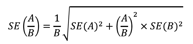
Let:
If the value under the square root sign is negative, then instead use
If P = 1 then use
- Means and Other Ratios
- Products
Users may combine these procedures for complicated estimates. For example, if the desired estimate is
then SE(A+B+C) and SE(D+E) can be estimated first, and then those results used to calculate SE(P).
For examples of these formulas, please see the 2005-2009 Accuracy of the Data, available at www.census.gov/acs/www/data_documentation/documentation_main/.
Once standard errors have been obtained, doing the statistical test to determine significance is not difficult. The determination of statistical significance takes into account the difference between the two estimates as well as the standard errors of both estimates.
For two estimates, A and B, with standard errors SE(A) and SE(B), let

If Z < -1.645 or Z > 1.645, then the difference between A and B is significant at the 90 percent confidence level. Otherwise, the difference is not significant. This means that there is less than a 10 percent chance that the difference between these two estimates would be as large or larger by random chance alone.
Users may choose to apply a confidence level different from 90 percent to their tests of statistical significance. For example, if Z< -1.96 or Z> 1.96, then the difference between A and B is significant at the 95 percent confidence level.
This method can be used for any types of estimates: counts, percentages, proportions, means, medians, etc. It can be used for comparing across years, or across surveys. If one of the estimates is a fixed value or comes from a source without sampling error (such as the Census 2000 SF1), use zero for the standard error for that estimate in the above equation for Z.
Using the rule of thumb of overlapping confidence intervals does not constitute a valid significance test and users are discouraged from using that method.
For two estimates, A and B, with standard errors SE(A) and SE(B), let
If Z < -1.645 or Z > 1.645, then the difference between A and B is significant at the 90 percent confidence level. Otherwise, the difference is not significant. This means that there is less than a 10 percent chance that the difference between these two estimates would be as large or larger by random chance alone.
Users may choose to apply a confidence level different from 90 percent to their tests of statistical significance. For example, if Z< -1.96 or Z> 1.96, then the difference between A and B is significant at the 95 percent confidence level.
This method can be used for any types of estimates: counts, percentages, proportions, means, medians, etc. It can be used for comparing across years, or across surveys. If one of the estimates is a fixed value or comes from a source without sampling error (such as the Census 2000 SF1), use zero for the standard error for that estimate in the above equation for Z.
Using the rule of thumb of overlapping confidence intervals does not constitute a valid significance test and users are discouraged from using that method.

