


| Documentation: | ACS 2012 (1-Year Estimates) |
| Document: | ACS 2012-1yr Summary File: Technical Documentation |
| citation: | Social Explorer; U.S. Census Bureau; American Community Survey 2012 Summary File: Technical Documentation. |
| Ancestry Code List | |
| Code | Write-In |
| 001-099 | WESTERN EUROPE (EXCEPT SPAIN) |
| 001 | ALSATIAN |
| 002 | ANDORRAN |
| 003 | AUSTRIAN |
| 004 | TIROL |
| 005 | BASQUE |
| 006 | FRENCH BASQUE |
| 007 | SPANISH BASQUE |
| 008 | BELGIAN |
| 009 | FLEMISH |
| 010 | WALLOON |
| 011 | BRITISH |
| 012 | BRITISH ISLES |
| 013 | CHANNEL ISLANDER |
| 014 | GIBRALTAR |
| 015 | CORNISH |
| 016 | CORSICAN |
| 017 | CYPRIOT |
| 018 | GREEK CYPRIOTE |
| 019 | TURKISH CYPRIOTE |
| 020 | DANISH |
| 021 | DUTCH |
| 022 | ENGLISH |
| 023 | FAROE ISLANDER |
| 024 | FINNISH |
| 025 | KARELIAN |
| 026 | FRENCH |
| 027 | LORRAINE |
| 028 | BRETON |
| 029 | FRISIAN |
| 030 | FRIULIAN |
| 031 | LADIN |
| 032 | GERMAN |
| 033 | BAVARIA |
| 034 | BERLIN |
| 035 | HAMBURG |
| 036 | HANNOVER |
| 037 | HESSIAN |
| 038 | LUBECKER |
| 039 | POMERANIAN |
| 040 | PRUSSIAN |
| 041 | SAXON |
| 042 | SUDETENLANDER |
| 043 | WESTPHALIAN |
| 044 | EAST GERMAN |
| 045 | WEST GERMAN |
| 046 | GREEK |
| 047 | CRETAN |
| 048 | CYCLADES |
| 049 | ICELANDER |
| 050 | IRISH |
| 051 | ITALIAN |
| 052 | TRIESTE |
| 053 | ABRUZZI |
| 054 | APULIAN |
| 055 | BASILICATA |
| 056 | CALABRIAN |
| 057 | AMALFIN |
| 058 | EMILIA ROMAGNA |
| 059 | ROME |
| 060 | LIGURIAN |
| 061 | LOMBARDIAN |
| 062 | MARCHE |
| 063 | MOLISE |
| 064 | NEAPOLITAN |
| 065 | PIEDMONTESE |
| 066 | PUGLIA |
| 067 | SARDINIAN |
| 068 | SICILIAN |
| 069 | TUSCANY |
| 070 | TRENTINO |
| 071 | UMBRIAN |
| 072 | VALLE DAOST |
| 073 | VENETIAN |
| 074 | SANMARINO |
| 075 | LAPP |
| 076 | LIECHTENSTEINER |
| 077 | LUXEMBURGER |
| 078 | MALTESE |
| 079 | MANX |
| 080 | MONEGASQUE |
| 081 | NORTH IRISH |
| 082 | NORWEGIAN |
| 083 | OCCITAN |
| 084 | PORTUGUESE |
| 085 | AZORES ISLANDER |
| 086 | MADEIRA ISLANDER |
| 087 | SCOTCH IRISH |
| 088 | SCOTTISH |
| 089 | SWEDISH |
| 090 | ALAND ISLANDER |
| 091 | SWISS |
| 092 | SUISSE |
| 093 | SWITZER |
| 094 | IRISH SCOTCH |
| 095 | ROMANSCH |
| 096 | SUISSE ROMANE |
| 097 | WELSH |
| 098 | SCANDINAVIAN |
| 099 | CELTIC |
| 100-180 | EASTERN EUROPE AND SOVIET UNION |
| 100 | ALBANIAN |
| 101 | AZERBAIJANI |
| 102 | BELORUSSIAN |
| 103 | BULGARIAN |
| 104 | CARPATHO RUSYN |
| 105 | CARPATHIAN |
| 106 | RUSYN |
| 107 | RUTHENIAN |
| 108 | COSSACK |
| 109 | CROATIAN |
| 110 | NOT USED |
| 111 | CZECH |
| 112 | BOHEMIAN |
| 113 | MORAVIAN |
| 114 | CZECHOSLOVAKIAN |
| 115 | ESTONIAN |
| 116 | LIVONIAN |
| 117 | FINNOUGRIAN |
| 118 | MORDOVIAN |
| 119 | VOYTAK |
| 120 | GRUZIIA |
| 121 | NOT USED |
| 122 | GERMAN FROM RUSSIA |
| 123 | VOLGA |
| 124 | ROM |
| 125 | HUNGARIAN |
| 126 | MAGYAR |
| 127 | KALMYK |
| 128 | LATVIAN |
| 129 | LITHUANIAN |
| 130 | MACEDONIAN |
| 131 | MONTENEGRIN |
| 132 | NORTH CAUCASIAN |
| 133 | NORTH CAUCASIAN TURKIC |
| 134-139 | NOT USED |
| 140 | OSSETIAN |
| 141 | NOT USED |
| 142 | POLISH |
| 143 | KASHUBIAN |
| 144 | ROMANIAN |
| 145 | BESSARABIAN |
| 146 | MOLDAVIAN |
| 147 | WALLACHIAN |
| 148 | RUSSIAN |
| 149 | NOT USED |
| 150 | MUSCOVITE |
| 151 | NOT USED |
| 152 | SERBIAN |
| 153 | SLOVAK |
| 154 | SLOVENE |
| 155 | SORBIAN/WEND |
| 156 | SOVIET TURKIC |
| 157 | BASHKIR |
| 158 | CHUVASH |
| 159 | GAGAUZ |
| 160 | MESKNETIAN |
| 161 | TUVINIAN |
| 162 | NOT USED |
| 163 | YAKUT |
| 164 | SOVIET UNION |
| 165 | TATAR |
| 166 | NOT USED |
| 167 | SOVIET CENTRAL ASIA |
| 168 | TURKESTANI |
| 169 | UZBEG |
| 170 | GEORGIA CIS |
| 171 | UKRAINIAN |
| 172 | LEMKO |
| 173 | BIOKO |
| 174 | HUSEL |
| 175 | WINDISH |
| 176 | YUGOSLAVIAN |
| 177 | HERZEGOVINIAN |
| 178 | SLAVIC |
| 179 | SLAVONIAN |
| 180 | TAJIK |
| 181-199 | EUROPE, N.E.C. |
| 181 | CENTRAL EUROPEAN |
| 182 | NOT USED |
| 183 | NORTHERN EUROPEAN |
| 184 | NOT USED |
| 185 | SOUTHERN EUROPEAN |
| 186 | NOT USED |
| 187 | WESTERN EUROPEAN |
| 188-189 | NOT USED |
| 190 | EASTERN EUROPEAN |
| 191 | BUKOVINA |
| 192 | NOT USED |
| 193 | SILESIAN |
| 194 | GERMANIC |
| 195 | EUROPEAN |
| 196 | GALICIAN |
| 197-199 | NOT USED |
| 200-299 | HISPANIC CATEGORIES (INCLUDING SPAIN) |
| 200 | SPANIARD |
| 201 | ANDALUSIAN |
| 202 | ASTURIAN |
| 203 | CASTILLIAN |
| 204 | CATALONIAN |
| 205 | BALEARIC ISLANDER |
| 206 | GALLEGO |
| 207 | VALENCIAN |
| 208 | CANARY ISLANDER |
| 209 | NOT USED |
| 210 | MEXICAN |
| 211 | MEXICAN AMERICAN |
| 212 | MEXICANO |
| 213 | CHICANO |
| 214 | LARAZA |
| 215 | MEXICAN AMERICAN INDIAN |
| 216-217 | NOT USED |
| 218 | MEXICAN STATE |
| 219 | MEXICAN INDIAN |
| 220 | NOT USED |
| 221 | COSTA RICAN |
| 222 | GUATEMALAN |
| 223 | HONDURAN |
| 224 | NICARAGUAN |
| 225 | PANAMANIAN |
| 226 | SALVADORAN |
| 227 | CENTRAL AMERICAN |
| 228 | NOT USED |
| 229 | CANAL ZONE |
| 230 | NOT USED |
| 231 | ARGENTINEAN |
| 232 | BOLIVIAN |
| 233 | CHILEAN |
| 234 | COLOMBIAN |
| 235 | ECUADORIAN |
| 236 | PARAGUAYAN |
| 237 | PERUVIAN |
| 238 | URUGUAYAN |
| 239 | VENEZUELAN |
| 240-247 | NOT USED |
| 248 | CRIOLLO |
| 249 | SOUTH AMERICAN |
| 250 | LATIN AMERICAN |
| 251 | LATIN |
| 252 | LATINO |
| 253-260 | NOT USED |
| 261 | PUERTO RICAN |
| 262-270 | NOT USED |
| 271 | CUBAN |
| 272-274 | NOT USED |
| 275 | DOMINICAN |
| 276-289 | NOT USED |
| 290 | HISPANIC |
| 291 | SPANISH |
| 292 | CALIFORNIO |
| 293 | TEJANO |
| 294 | NUEVO MEXICANO |
| 295 | SPANISH AMERICAN |
| 296-299 | NOT USED |
| 300-359 | WEST INDIES (EXCEPT HISPANIC) |
| 300 | BAHAMIAN |
| 301 | BARBADIAN |
| 302 | BELIZEAN |
| 303 | BERMUDAN |
| 304 | CAYMAN ISLANDER |
| 305-307 | NOT USED |
| 308 | JAMAICAN |
| 309 | NOT USED |
| 310 | DUTCH WEST INDIES |
| 311 | ARUBA ISLANDER |
| 312 | ST MAARTEN ISLANDER |
| 313 | NOT USED |
| 314 | TRINIDADIAN TOBAGONIAN |
| 315 | TRINIDADIAN |
| 316 | TOBAGONIAN |
| 317 | U S VIRGIN ISLANDER |
| 318 | ST CROIX ISLANDER |
| 319 | ST JOHN ISLANDER |
| 320 | ST THOMAS ISLANDER |
| 321 | BRITISH VIRGIN ISLANDER |
| 322 | BRITISH WEST INDIES |
| 323 | TURKS AND CAICOS ISLANDER |
| 324 | ANGUILLA ISLANDER |
| 325 | ANTIGUA AND BARBUDA |
| 326 | MONTSERRAT ISLANDER |
| 327 | KITTS/NEVIS ISLANDER |
| 328 | DOMINICA ISLANDER |
| 329 | GRENADIAN |
| 330 | VINCENT GRENADINE ISLANDER |
| 331 | ST LUCIA ISLANDER |
| 332 | FRENCH WEST INDIES |
| 333 | GUADELOUPE ISLANDER |
| 334 | CAYENNE |
| 335 | WEST INDIAN |
| 336 | HAITIAN |
| 337-359 | NOT USED |
| 360-399 | CENTRAL AND SOUTH AMERICA (EXCEPT HISPANIC) |
| 360 | BRAZILIAN |
| 361-364 | NOT USED |
| 365 | SAN ANDRES |
| 366-369 | NOT USED |
| 370 | GUYANESE |
| 371-374 | NOT USED |
| 375 | PROVIDENCIA |
| 376-379 | NOT USED |
| 380 | SURINAM |
| 381-399 | NOT USED |
| 400-499 | NORTH AFRICA AND SOUTH WEST ASIA |
| 400 | ALGERIAN |
| 401 | NOT USED |
| 402 | EGYPTIAN |
| 403 | NOT USED |
| 404 | LIBYAN |
| 405 | NOT USED |
| 406 | MOROCCAN |
| 407 | IFNI |
| 408 | TUNISIAN |
| 409-410 | NOT USED |
| 411 | NORTH AFRICAN |
| 412 | ALHUCEMAS |
| 413 | BERBER |
| 414 | RIO DE ORO |
| 415 | BAHRAINI |
| 416 | IRANIAN |
| 417 | IRAQI |
| 418 | NOT USED |
| 419 | ISRAELI |
| 420 | NOT USED |
| 421 | JORDANIAN |
| 422 | TRANSJORDAN |
| 423 | KUWAITI |
| 424 | NOT USED |
| 425 | LEBANESE |
| 426 | NOT USED |
| 427 | SAUDI ARABIAN |
| 428 | NOT USED |
| 429 | SYRIAN |
| 430 | NOT USED |
| 431 | ARMENIAN |
| 432-433 | NOT USED |
| 434 | TURKISH |
| 435 | YEMENI |
| 436 | OMANI |
| 437 | MUSCAT |
| 438 | TRUCIAL STATES |
| 439 | QATAR |
| 440 | NOT USED |
| 441 | BEDOUIN |
| 442 | KURDISH |
| 443 | NOT USED |
| 444 | KURIA MURIA ISLANDER |
| 445-464 | NOT USED |
| 465 | PALESTINIAN |
| 466 | GAZA STRIP |
| 467 | WEST BANK |
| 468-469 | NOT USED |
| 470 | SOUTH YEMEN |
| 471 | ADEN |
| 472-479 | NOT USED |
| 480 | UNITED ARAB EMIRATES |
| 481 | NOT USED |
| 483 | ASSYRIAN |
| 484 | CHALDEAN |
| 485 | SYRIAC |
| 486-489 | NOT USED |
| 490 | MIDEAST |
| 491-494 | NOT USED |
| 495 | ARAB |
| 496 | ARABIC |
| 497-499 | NOT USED |
| 500-599 | SUBSAHARAN AFRICA |
| 500 | ANGOLAN |
| 501 | NOT USED |
| 502 | BENIN |
| 503 | NOT USED |
| 504 | BOTSWANA |
| 505 | NOT USED |
| 506 | BURUNDIAN |
| 507 | NOT USED |
| 508 | CAMEROON |
| 509 | NOT USED |
| 510 | CAPE VERDEAN |
| 511 | NOT USED |
| 512 | CENTRAL AFRICAN REPUBLIC |
| 513 | CHADIAN |
| 514 | NOT USED |
| 515 | CONGOLESE |
| 516 | CONGO BRAZZAVILLE |
| 517-518 | NOT USED |
| 519 | DJIBOUTI |
| 520 | EQUATORIAL GUINEA |
| 521 | CORSICO ISLANDER |
| 522 | ETHIOPIAN |
| 523 | ERITREAN |
| 524 | NOT USED |
| 525 | GABONESE |
| 526 | NOT USED |
| 527 | GAMBIAN |
| 528 | NOT USED |
| 529 | GHANAIAN |
| 530 | GUINEAN |
| 531 | GUINEA BISSAU |
| 532 | IVORY COAST |
| 533 | NOT USED |
| 534 | KENYAN |
| 535-537 | NOT USED |
| 538 | LESOTHO |
| 539-540 | NOT USED |
| 541 | LIBERIAN |
| 542 | NOT USED |
| 543 | MADAGASCAN |
| 544 | NOT USED |
| 545 | MALAWIAN |
| 546 | MALIAN |
| 547 | MAURITANIAN |
| 548 | NOT USED |
| 549 | MOZAMBICAN |
| 550 | NAMIBIAN |
| 551 | NIGER |
| 552 | NOT USED |
| 553 | NIGERIAN |
| 554 | FULANI |
| 555 | HAUSA |
| 556 | IBO |
| 557 | TIV |
| 558 | YORUBA |
| 559-560 | NOT USED |
| 561 | RWANDAN |
| 562-563 | NOT USED |
| 564 | SENEGALESE |
| 565 | NOT USED |
| 566 | SIERRA LEONEAN |
| 567 | NOT USED |
| 568 | SOMALIAN |
| 569 | SWAZILAND |
| 570 | SOUTH AFRICAN |
| 571 | UNION OF SOUTH AFRICA |
| 572 | AFRIKANER |
| 573 | NATALIAN |
| 574 | ZULU |
| 575 | NOT USED |
| 576 | SUDANESE |
| 577 | DINKA |
| 578 | NUER |
| 579 | FUR |
| 580 | BAGGARA |
| 581 | NOT USED |
| 582 | TANZANIAN |
| 583 | TANGANYIKAN |
| 584 | ZANZIBAR ISLANDER |
| 585 | NOT USED |
| 586 | TOGO |
| 587 | NOT USED |
| 588 | UGANDAN |
| 589 | UPPER VOLTAN |
| 590 | VOLTA |
| 591 | ZAIRIAN |
| 592 | ZAMBIAN |
| 593 | ZIMBABWEAN |
| 594 | AFRICAN ISLANDS (EXCEPT MADAGASCAR) |
| 595 | MAURITIAN |
| 596 | CENTRAL AFRICAN |
| 597 | EASTERN AFRICAN |
| 598 | WESTERN AFRICAN |
| 599 | AFRICAN |
| 600-699 | SOUTH ASIA |
| 600 | AFGHANISTAN |
| 601 | BALUCHISTAN |
| 602 | PATHAN |
| 603 | BANGLADESHI |
| 604-606 | NOT USED |
| 607 | BHUTANESE |
| 608 | NOT USED |
| 609 | NEPALI |
| 610-614 | NOT USED |
| 615 | ASIAN INDIAN |
| 616 | KASHMIR |
| 617 | NOT USED |
| 618 | BENGALI |
| 619 | NOT USED |
| 620 | EAST INDIAN |
| 621 | NOT USED |
| 622 | ANDAMAN ISLANDER |
| 623 | NOT USED |
| 624 | ANDHRA PRADESH |
| 625 | NOT USED |
| 626 | ASSAMESE |
| 627 | NOT USED |
| 628 | GOANESE |
| 629 | NOT USED |
| 630 | GUJARATI |
| 631 | NOT USED |
| 632 | KARNATAKAN |
| 633 | NOT USED |
| 634 | KERALAN |
| 635 | NOT USED |
| 636 | MADHYA PRADESH |
| 637 | NOT USED |
| 638 | MAHARASHTRAN |
| 639 | NOT USED |
| 640 | MADRAS |
| 641 | NOT USED |
| 642 | MYSORE |
| 643 | NOT USED |
| 644 | NAGALAND |
| 645 | NOT USED |
| 646 | ORISSA |
| 647 | NOT USED |
| 648 | PONDICHERRY |
| 649 | NOT USED |
| 650 | PUNJAB |
| 651 | NOT USED |
| 652 | RAJASTHAN |
| 653 | NOT USED |
| 654 | SIKKIM |
| 655 | NOT USED |
| 656 | TAMIL NADU |
| 657 | NOT USED |
| 658 | UTTAR PRADESH |
| 659-674 | NOT USED |
| 675 | EASTINDIES |
| 676-679 | NOT USED |
| 680 | PAKISTANI |
| 681-689 | NOT USED |
| 690 | SRILANKAN |
| 691 | SINGHALESE |
| 692 | VEDDAH |
| 693-694 | NOT USED |
| 695 | MALDIVIAN |
| 696-699 | NOT USED |
| 700-799 | OTHER ASIA |
| 700 | BURMESE |
| 701 | NOT USED |
| 702 | SHAN |
| 703 | CAMBODIAN |
| 704 | KHMER |
| 705 | NOT USED |
| 706 | CHINESE |
| 707 | CANTONESE |
| 708 | MANCHURIAN |
| 709 | MANDARIN |
| 710-711 | NOT USED |
| 712 | MONGOLIAN |
| 713 | NOT USED |
| 714 | TIBETAN |
| 715 | NOT USED |
| 716 | HONG KONG |
| 717 | NOT USED |
| 718 | MACAO |
| 719 | NOT USED |
| 720 | FILIPINO |
| 721-729 | NOT USED |
| 730 | INDONESIAN |
| 731 | NOT USED |
| 732 | BORNEO |
| 733 | NOT USED |
| 734 | JAVA |
| 735 | NOT USED |
| 736 | SUMATRA |
| 737-739 | NOT USED |
| 740 | JAPANESE |
| 741 | ISSEI |
| 742 | NISEI |
| 743 | SANSEI |
| 744 | YONSEI |
| 745 | GONSEI |
| 746 | RYUKYU ISLANDER |
| 747 | NOT USED |
| 748 | OKINAWAN |
| 749 | NOT USED |
| 750 | KOREAN |
| 751-764 | NOT USED |
| 765 | LAOTIAN |
| 766 | MEO |
| 767 | NOT USED |
| 768 | HMONG |
| 769 | NOT USED |
| 770 | MALAYSIAN |
| 771 | NORTH BORNEO |
| 772-773 | NOT USED |
| 774 | SINGAPOREAN |
| 775 | NOT USED |
| 776 | THAI |
| 777 | BLACK THAI |
| 778 | WESTERN LAO |
| 779-781 | NOT USED |
| 782 | TAIWANESE |
| 783 | FORMOSAN |
| 784 | NOT USED |
| 785 | VIETNAMESE |
| 786 | KATU |
| 787 | MA |
| 788 | MNONG |
| 789 | NOT USED |
| 790 | MONTAGNARD |
| 791 | NOT USED |
| 792 | INDO CHINESE |
| 793 | EURASIAN |
| 794 | AMERASIAN |
| 795 | ASIAN |
| 796-799 | NOT USED |
| 800-899 | PACIFIC |
| 800 | AUSTRALIAN |
| 801 | TASMANIAN |
| 802 | AUSTRALIAN ABORIGINE |
| 803 | NEW ZEALANDER |
| 804 | TUVALUAN |
| 805 | NORFOLK ISLANDER |
| 806-807 | NOT USED |
| 808 | POLYNESIAN |
| 809 | KAPINGAMARANGAN |
| 810 | MAORI |
| 811 | HAWAIIAN |
| 812 | NOT USED |
| 813 | PART HAWAIIAN |
| 814 | SAMOAN |
| 815 | TONGAN |
| 816 | TOKELAUAN |
| 817 | COOK ISLANDER |
| 818 | TAHITIAN |
| 819 | NIUEAN |
| 820 | MICRONESIAN |
| 821 | GUAMANIAN |
| 822 | CHAMORRO ISLANDER |
| 823 | SAIPANESE |
| 824 | PALAUAN |
| 825 | MARSHALLESE |
| 826 | KOSRAEAN |
| 827 | PONAPEAN |
| 828 | TRUKESE (CHUUKESE) |
| 829 | YAPESE |
| 830 | CAROLINIAN |
| 831 | KIRIBATESE |
| 832 | NAURUAN |
| 833 | TARAWA ISLANDER |
| 834 | TINIAN ISLANDER |
| 835-839 | NOT USED |
| 840 | MELANESIAN |
| 841 | FIJIAN |
| 842 | NOT USED |
| 843 | NEW GUINEAN |
| 844 | PAPUAN |
| 845 | SOLOMON ISLANDER |
| 846 | NEW CALEDONIAN |
| 847 | VANUATUAN |
| 848-849 | NOT USED |
| 850 | PACIFIC ISLANDER |
| 851-859 | NOT USED |
| 860 | PACIFIC |
| 861 | NOT USED |
| 862 | CHAMOLINIAN |
| 863-899 | NOT USED |
| 900-994 | NORTH AMERICA (EXCEPT HISPANIC) |
| 900 | AFRO AMERICAN |
| 901 | AFRO |
| 902 | AFRICAN AMERICAN |
| 903 | BLACK |
| 904 | NEGRO |
| 905 | NONWHITE |
| 906 | COLORED |
| 907 | CREOLE |
| 908 | MULATTO |
| 909- | NOT USED |
| 913 | CENTRAL AMERICAN INDIAN |
| 914 | SOUTH AMERICAN INDIAN |
| 915- | NOT USED |
| 917 | NATIVE AMERICAN |
| 918 | INDIAN |
| 919 | CHEROKEE |
| 920 | AMERICAN INDIAN |
| 921 | ALEUT |
| 922 | ESKIMO |
| 923 | INUIT |
| 924 | WHITE |
| 925 | ANGLO |
| 926 | NOT USED |
| 927 | APPALACHIAN |
| 928 | ARYAN |
| 929 | PENNSYLVANIA GERMAN |
| 930 | GREENLANDER |
| 931 | CANADIAN |
| 932 | NOT USED |
| 933 | NEWFOUNDLAND |
| 934 | NOVA SCOTIA |
| 935 | FRENCH CANADIAN |
| 936 | ACADIAN |
| 937 | CAJUN |
| 938 | NOT USED |
| 939 | AMERICAN |
| 940 | UNITED STATES |
| 941 | ALABAMA |
| 942 | ALASKA |
| 943 | ARIZONA |
| 944 | ARKANSAS |
| 945 | CALIFORNIA |
| 946 | COLORADO |
| 947 | CONNECTICUT |
| 948 | DISTRICT OF COLUMBIA |
| 949 | DELAWARE |
| 950 | FLORIDA |
| 951 | IDAHO |
| 952 | ILLINOIS |
| 953 | INDIANA |
| 954 | IOWA |
| 955 | KANSAS |
| 956 | KENTUCKY |
| 957 | LOUISIANA |
| 958 | MAINE |
| 959 | MARYLAND |
| 960 | MASSACHUSETTS |
| 961 | MICHIGAN |
| 962 | MINNESOTA |
| 963 | MISSISSIPPI |
| 964 | MISSOURI |
| 965 | MONTANA |
| 966 | NEBRASKA |
| 967 | NEVADA |
| 968 | NEW HAMPSHIRE |
| 969 | NEW JERSEY |
| 970 | NEW MEXICO |
| 971 | NEW YORK |
| 972 | NORTH CAROLINA |
| 973 | NORTH DAKOTA |
| 974 | OHIO |
| 975 | NOT USED |
| 976 | OKLAHOMA |
| 977 | OREGON |
| 978 | PENNSYLVANIA |
| 979 | RHODE ISLAND |
| 980 | SOUTH CAROLINA |
| 981 | SOUTH DAKOTA |
| 982 | TENNESSEE |
| 983 | TEXAS |
| 984 | UTAH |
| 985 | VERMONT |
| 986 | VIRGINIA |
| 987 | WASHINGTON |
| 988 | WEST VIRGINIA |
| 989 | WISCONSIN |
| 990 | WYOMING |
| 991 | GEORGIA |
| 992 | NOT USED |
| 993 | SOUTHERNER |
| 994 | NORTH AMERICAN |
| 995-999 | RESIDUAL AND NORESPONSE |
| 995 | MIXTURE |
| 996 | UNCODABLE ENTRIES |
| 997 | NOT USED |
| 998 | OTHER RESPONSES |
| 999 | NOT REPORTED |
Institutional Group Quarters: |
| Correctional facilities for adults |
| 101. Federal detention centers |
| 102. Federal prisons |
| 103. State prisons |
| 104. Local jails and other municipal confinement facilities |
| 105. Correctional residential facilities |
| 106. Military disciplinary barracks and jails |
| Juvenile facilities |
| 201. Group homes for juveniles (non-correctional) |
| 202. Residential treatment centers for juveniles (non-correctional) |
| 203. Correctional facilities intended for juveniles |
| Nursing facilities/skilled-nursing facilities |
| 301. Nursing facilities/skilled-nursing facilities |
| Other institutional facilities |
| 401. Mental (psychiatric) hospitals and psychiatric units in other hospitals |
| 402. Hospitals with patients who have no usual home elsewhere |
| 403. In-patient hospice facilities |
| 404. Military treatment facilities with assigned patients |
| 405. Residential schools for people with disabilities |
Noninstitutional Group Quarters: |
| College/university student housing |
| 501. College/university student housing |
| Military Quarters |
| 601. Military quarters |
| 602. Military ships |
| Other noninstitutional facilities |
| 701. Emergency and transitional shelters (with sleeping facilities) for people experiencing homelessness |
| 801. Group homes intended for adults |
| 802. Residential treatment centers for adults |
| 901. Workers' group living quarters and Job Corps centers |
| 902. Religious group quarters |
001-199, 300-999 Not Spanish/Hispanic | 200-209 Spaniard | 210-220 Mexican |
| 221-230 Central American | 231-249 South American | 250-259 Latin American |
| 260-269 Puerto Rican | 270-274 Cuban | 275-279 Dominican |
280-299 Other Spanish/Hispanic | ||
| 001-199 Not Spanish/Hispanic | ||
| 001-099 Not used | 100 Not Hispanic/Spanish (CHECK BOX) | 101 Not Hispanic/Spanish |
| 102-109 Not Used | 110 Portuguese | 111 Azorean |
| 112 Brazilian | 113-115 Not Used | 116 Belizean |
| 117 British Honduran | 118 Haitian | 119 Dominica Island |
| 120 Basque | 121 Sephardic | 122-129 Not used |
| 130 White | 131-134 Not used | 135 Black (African American) |
| 136-144 Not used | 145 American Indian | 146 Alaska Native |
| 147-149 Not used | 150 Other Asian | 151 Asian Indian |
| 152 Chinese | 153 Filipino | 154 Japanese |
| 155 Korean | 156 Vietnamese | 157-159 Not used |
| 160 Native Hawaiian | 161-165 Not used | 166 Other Pacific Islander |
| 167 Guamanian or Chamorro | 168 Samoan | 169-199 Not used |
| 200-209 Spaniard | ||
| 200 Spaniard | 201 Andalusian | 202 Asturian |
| 203 Castillian | 204 Catalonian | 205 Balearic Islander |
| 206 Gallego | 207 Valencian | 208 Canarian |
| 209 Spanish Basque | ||
| 210-220 Mexican | ||
| 210 Mexican (CHECK BOX) | 211 Mexican | 212 Mexican American |
| 213 Mexicano | 214 Chicano | 215 La Raza |
| 216 Mexican American Indian | 217 Not Used | 218 Mexican State |
| 219 Mexican Indian | 220 Not Used | |
| 221-230 Central American | ||
| 221 Costa Rican | 222 Guatemalan | 223 Honduran |
| 224 Nicaraguan | 225 Panamanian | 226 Salvadoran |
| 227 Central American | 228 Central American Indian | 229 Canal Zone |
| 230 Not Used | ||
| 231-249 South American | ||
| 231 Argentinean | 232 Bolivian | 233 Chilean |
| 234 Colombian | 235 Ecuadorian | 236 Paraguayan |
| 237 Peruvian | 238 Uruguayan | 239 Venezuelan |
| 240 South American Indian | 241 Criollo | 242 South American |
| 243-249 Not Used | ||
| 250-259 Latin American | ||
| 250 Latin American | 251 Latin | 252 Latino |
| 253-259 Not Used | ||
| 260-269 Puerto Rican | ||
| 260 Puerto Rican (CHECK BOX) | 261 Puerto Rican | 262-269 Not Used |
| 270-274 Cuban | ||
| 270 Cuban (CHECK BOX) | 271 Cuban | 272-274 Not used |
| 275-279 Dominican | ||
| 275 Dominican | 276-279 Not Used | |
| 280-299 Other Spanish/Hispanic | ||
| 280 Other Spanish/Hispanic (CHECK BOX) | 281 Hispanic | 282 Spanish |
| 283 Californio | 284 Tejano | 285 Nuevo Mexicano |
| 286 Spanish American | 287 Spanish American Indian | 288 Meso American Indian |
| 289 Mestizo | 290 Caribbean | 291-298 Not Used |
| 299 Other Spanish/Hispanic, N.E.C. | ||
| Industry 2007 Description | 2007 Census Code | 2007 NAICS Code | |
| Agriculture, Forestry, Fishing, and Hunting, and Mining | 0170-0490 | 11-21 | |
| Agriculture, Forestry, Fishing, and Hunting | 0170-0290 | 11 | |
| Crop production | 0170 | 111 | |
| Animal production | 0180 | 112 | |
| Forestry except logging | 0190 | 1131, 1132 | |
| Logging | 0270 | 1133 | |
| Fishing, hunting and trapping | 0280 | 114 | |
| Support activities for agriculture and forestry | 0290 | 115 | |
| Mining, Quarrying, and Oil and Gas Extraction | 0370-0490 | 21 | |
| Oil and gas extraction | 0370 | 211 | |
| Coal mining | 0380 | 2121 | |
| Metal ore mining | 0390 | 2122 | |
| Nonmetallic mineral mining and quarrying | 0470 | 2123 | |
| Not specified type of mining | 0480 | Part of 21 | |
| Support activities for mining | 0490 | 213 | |
| Construction | 0770 | 23 | |
| Construction (the cleaning of buildings and dwellings is incidental during construction and immediately after construction) | 0770 | 23 | |
| Manufacturing | 1070-3990 | 31-33 | |
| Animal food, grain and oilseed milling | 1070 | 3111, 3112 | |
| Sugar and confectionery products | 1080 | 3113 | |
| Fruit and vegetable preserving and specialty food manufacturing | 1090 | 3114 | |
| Dairy product manufacturing | 1170 | 3115 | |
| Animal slaughtering and processing | 1180 | 3116 | |
| Retail bakeries | 1190 | 311811 | |
| Bakeries, except retail | 1270 | 3118 exc. 311811 | |
| Seafood and other miscellaneous foods, n.e.c. | 1280 | 3117, 3119 | |
| Not specified food industries | 1290 | Part of 311 | |
| Beverage manufacturing | 1370 | 3121 | |
| Tobacco manufacturing | 1390 | 3122 | |
| Fiber, yarn, and thread mills | 1470 | 3131 | |
| Fabric mills, except knitting mills | 1480 | 3132 exc. 31324 | |
| Textile and fabric finishing and fabric coating mills | 1490 | 3133 | |
| Carpet and rug mills | 1570 | 31411 | |
| Textile product mills, except carpet and rug | 1590 | 314 exc. 31411 | |
| Knitting fabric mills, and apparel knitting mills | 1670 | 31324, 3151 | |
| Cut and sew apparel manufacturing | 1680 | 3152 | |
| Apparel accessories and other apparel manufacturing | 1690 | 3159 | |
| Footwear manufacturing | 1770 | 3162 | |
| Leather tanning and finishing and other allied products manufacturing | 1790 | 3161, 3169 | |
| Pulp, paper, and paperboard mills | 1870 | 3221 | |
| Paperboard containers and boxes | 1880 | 32221 | |
| Miscellaneous paper and pulp products | 1890 | 32222,32223,32229 | |
| Printing and related support activities | 1990 | 3231 | |
| Petroleum refining | 2070 | 32411 | |
| Miscellaneous petroleum and coal products | 2090 | 32412,32419 | |
| Resin, synthetic rubber, and fibers and filaments manufacturing | 2170 | 3252 | |
| Agricultural chemical manufacturing | 2180 | 3253 | |
| Pharmaceutical and medicine manufacturing | 2190 | 3254 | |
| Paint, coating, and adhesive manufacturing | 2270 | 3255 | |
| Soap, cleaning compound, and cosmetics manufacturing | 2280 | 3256 | |
| Industrial and miscellaneous chemicals | 2290 | 3251, 3259 | |
| Plastics product manufacturing | 2370 | 3261 | |
| Tire manufacturing | 2380 | 32621 | |
| Rubber products, except tires, manufacturing | 2390 | 32622, 32629 | |
| Pottery, ceramics, and plumbing fixture manufacturing | 2470 | 32711 | |
| Structural clay product manufacturing | 2480 | 32712 | |
| Glass and glass product manufacturing | 2490 | 3272 | |
| Cement, concrete, lime, and gypsum product manufacturing | 2570 | 3273, 3274 | |
| Miscellaneous nonmetallic mineral product manufacturing | 2590 | 3279 | |
| Iron and steel mills and steel product manufacturing | 2670 | 3311, 3312 | |
| Aluminum production and processing | 2680 | 3313 | |
| Nonferrous metal (except aluminum) production and processing | 2690 | 3314 | |
| Foundries | 2770 | 3315 | |
| Metal forgings and stampings | 2780 | 3321 | |
| Cutlery and hand tool manufacturing | 2790 | 3322 | |
| Structural metals, and boiler, tank, and shipping container manufacturing | 2870 | 3323, 3324 | |
| Machine shops; turned product; screw, nut, and bolt manufacturing | 2880 | 3327 | |
| Coating, engraving, heat treating, and allied activities | 2890 | 3328 | |
| Ordnance | 2970 | 332992, 332993, 332994, 332995 | |
| Miscellaneous fabricated metal products manufacturing | 2980 | 3325, 3326, 3329 exc. 332992, 332993, 332994, 332995 | |
| Not specified metal industries | 2990 | Part of 331 and 332 | |
| Agricultural implement manufacturing | 3070 | 33311 | |
| Construction, and mining and oil and gas field machinery manufacturing | 3080 | 33312, 33313 | |
| Commercial and service industry machinery manufacturing | 3090 | 3333 | |
| Metalworking machinery manufacturing | 3170 | 3335 | |
| Engines, turbines, and power transmission equipment manufacturing | 3180 | 3336 | |
| Machinery manufacturing, n.e.c. | 3190 | 3332, 3334, 3339 | |
| Not specified machinery manufacturing | 3290 | Part of 333 | |
| Computer and peripheral equipment manufacturing | 3360 | 3341 | |
| Communications, and audio and video equipment manufacturing | 3370 | 3342, 3343 | |
| Navigational, measuring, electromedical, and control instruments manufacturing | 3380 | 3345 | |
| Electronic component and product manufacturing, n.e.c. | 3390 | 3344, 3346 | |
| Household appliance manufacturing | 3470 | 3352 | |
| Electric lighting and electrical equipment manufacturing, and other electrical component manufacturing, n.e.c. | 3490 | 3351, 3353, 3359 | |
| Motor vehicles and motor vehicle equipment manufacturing | 3570 | 3361, 3362, 3363 | |
| Aircraft and parts manufacturing | 3580 | 336411, 336412, 336413 | |
| Aerospace products and parts manufacturing | 3590 | 336414, 336415, 336419 | |
| Railroad rolling stock manufacturing | 3670 | 3365 | |
| Ship and boat building | 3680 | 3366 | |
| Other transportation equipment manufacturing | 3690 | 3369 | |
| Sawmills and wood preservation | 3770 | 3211 | |
| Veneer, plywood, and engineered wood products | 3780 | 3212 | |
| Prefabricated wood buildings and mobile homes | 3790 | 321991, 321992 | |
| Miscellaneous wood products | 3870 | 3219 exc. 321991, 321992 | |
| Furniture and related product manufacturing | 3890 | 337 | |
| Medical equipment and supplies manufacturing | 3960 | 3391 | |
| Sporting and athletic goods, and doll, toy and game manufacturing | 3970 | 33992, 33993 | |
| Miscellaneous manufacturing, n.e.c. | 3980 | 3399 exc. 33992, 33993 | |
| Not specified manufacturing industries | 3990 | Part of 31, 32, 33 | |
| Wholesale Trade | 4070-4590 | 42 | |
| Motor vehicles, parts and supplies merchant wholesalers | 4070 | 4231 | |
| Furniture and home furnishing merchant wholesalers | 4080 | 4232 | |
| Lumber and other construction materials merchant wholesalers | 4090 | 4233 | |
| Professional and commercial equipment and supplies merchant wholesalers | 4170 | 4234 | |
| Metals and minerals, except petroleum, merchant wholesalers | 4180 | 4235 | |
| Electrical and electronic goods merchant wholesalers | 4190 | 4236 | |
| Hardware, plumbing and heating equipment, and supplies merchant wholesalers | 4260 | 4237 | |
| Machinery, equipment, and supplies merchant wholesalers | 4270 | 4238 | |
| Recyclable material merchant wholesalers | 4280 | 42393 | |
| Miscellaneous durable goods merchant wholesalers | 4290 | 4239 exc. 42393 | |
| Paper and paper products merchant wholesalers | 4370 | 4241 | |
| Drugs, sundries, and chemical and allied products merchant wholesalers | 4380 | 4242, 4246 | |
| Apparel, fabrics, and notions merchant wholesalers | 4390 | 4243 | |
| Groceries and related products merchant wholesalers | 4470 | 4244 | |
| Farm product raw materials merchant wholesalers | 4480 | 4245 | |
| Petroleum and petroleum products merchant wholesalers | 4490 | 4247 | |
| Alcoholic beverages merchant wholesalers | 4560 | 4248 | |
| Farm supplies merchant wholesalers | 4570 | 42491 | |
| Miscellaneous nondurable goods merchant wholesalers | 4580 | 4249 exc. 42491 | |
| Wholesale electronic markets and agents and brokers | 4585 | 4251 | |
| Not specified wholesale trade | 4590 | Part of 42 | |
| Retail Trade | 4670-5790 | 44-45 | |
| Automobile dealers | 4670 | 4411 | |
| Other motor vehicle dealers | 4680 | 4412 | |
| Auto parts, accessories, and tire stores | 4690 | 4413 | |
| Furniture and home furnishings stores | 4770 | 442 | |
| Household appliance stores | 4780 | 443111 | |
| Radio, TV, and computer stores | 4790 | 443112, 44312 | |
| Building material and supplies dealers | 4870 | 4441 exc. 44413 | |
| Hardware stores | 4880 | 44413 | |
| Lawn and garden equipment and supplies stores | 4890 | 4442 | |
| Grocery stores | 4970 | 4451 | |
| Specialty food stores | 4980 | 4452 | |
| Beer, wine, and liquor stores | 4990 | 4453 | |
| Pharmacies and drug stores | 5070 | 44611 | |
| Health and personal care, except drug, stores | 5080 | 446 exc. 44611 | |
| Gasoline stations | 5090 | 447 | |
| Clothing stores | 5170 | 4481 | |
| Shoe stores | 5180 | 44821 | |
| Jewelry, luggage, and leather goods stores | 5190 | 4483 | |
| Sporting goods, camera, and hobby and toy stores | 5270 | 44313, 45111, 45112 | |
| Sewing, needlework, and piece goods stores | 5280 | 45113 | |
| Music stores | 5290 | 45114, 45122 | |
| Book stores and news dealers | 5370 | 45121 | |
| Department stores and discount stores | 5380 | 45211 | |
| Miscellaneous general merchandise stores | 5390 | 4529 | |
| Retail florists | 5470 | 4531 | |
| Office supplies and stationery stores | 5480 | 45321 | |
| Used merchandise stores | 5490 | 4533 | |
| Gift, novelty, and souvenir shops | 5570 | 45322 | |
| Miscellaneous retail stores | 5580 | 4539 | |
| Electronic shopping | 5590 | 454111 | |
| Electronic auctions | 5591 | 454112 | |
| Mail order houses | 5592 | 454113 | |
| Vending machine operators | 5670 | 4542 | |
| Fuel dealers | 5680 | 45431 | |
| Other direct selling establishments | 5690 | 45439 | |
| Not specified retail trade | 5790 | Part of 44, 45 | |
| Transportation and Warehousing and Utilities | 6070-6390, 0570-0690 | 48-49, 22 | |
| Transportation and Warehousing | 6070-6390 | 48-49 | |
| Air transportation | 6070 | 481 | |
| Rail transportation | 6080 | 482 | |
| Water transportation | 6090 | 483 | |
| Truck transportation | 6170 | 484 | |
| Bus service and urban transit | 6180 | 4851, 4852, 4854, 4855, 4859 | |
| Taxi and limousine service | 6190 | 4853 | |
| Pipeline transportation | 6270 | 486 | |
| Scenic and sightseeing transportation | 6280 | 487 | |
| Services incidental to transportation | 6290 | 488 | |
| Postal Service | 6370 | 491 | |
| Couriers and messengers | 6380 | 492 | |
| Warehousing and storage | 6390 | 493 | |
| Utilities | 0570-0690 | 22 | |
| Electric power generation, transmission and distribution | 0570 | 2211 | |
| Natural gas distribution | 0580 | 2212 | |
| Electric and gas, and other combinations | 0590 | Pts. 2211, 2212 | |
| Water, steam, air-conditioning, and irrigation systems | 0670 | 22131, 22133 | |
| Sewage treatment facilities | 0680 | 22132 | |
| Not specified utilities | 0690 | Part of 22 | |
| Information | 6470-6780 | 51 | |
| Newspaper publishers | 6470 | 51111 | |
| Periodical, book, and directory publishers | 6480 | 5111 exc. 51111 | |
| Software publishers | 6490 | 5112 | |
| Motion picture and video industries | 6570 | 5121 | |
| Sound recording industries | 6590 | 5122 | |
| Radio and television broadcasting and cable subscription programming | 6670 | 515 | |
| Internet publishing and broadcasting and web search portals | 6672 | 51913 | |
| Wired telecommunications carriers | 6680 | 5171 | |
| Other telecommunications services | 6690 | 517 exc. 5171 | |
| Data processing, hosting, and related services | 6695 | 5182 | |
| Libraries and archives | 6770 | 51912 | |
| Other information services | 6780 | 5191 exc. 51912, 51913 | |
| Finance and Insurance, and Real Estate, and Rental and Leasing | 6870-7190 | 52-53 | |
| Finance and Insurance | 6870-6990 | 52 | |
| Banking and related activities | 6870 | 521, 52211,52219 | |
| Savings institutions, including credit unions | 6880 | 52212, 52213 | |
| Non-depository credit and related activities | 6890 | 5222, 5223 | |
| Securities, commodities, funds, trusts, and other financial investments | 6970 | 523, 525 | |
| Insurance carriers and related activities | 6990 | 524 | |
| Real Estate and Rental and Leasing | 7070-7190 | 53 | |
| Real estate | 7070 | 531 | |
| Automotive equipment rental and leasing | 7080 | 5321 | |
| Video tape and disk rental | 7170 | 53223 | |
| Other consumer goods rental | 7180 | 53221, 53222, 53229, 5323 | |
| Commercial, industrial, and other intangible assets rental and leasing | 7190 | 5324, 533 | |
| Professional, Scientific, and Management, and Administrative, and Waste Management Services | 7270-7790 | 54-56 | |
| Professional, Scientific, and Technical Services | 7270-7490 | 54 | |
| Legal services | 7270 | 5411 | |
| Accounting, tax preparation, bookkeeping, and payroll services | 7280 | 5412 | |
| Architectural, engineering, and related services | 7290 | 5413 | |
| Specialized design services | 7370 | 5414 | |
| Computer systems design and related services | 7380 | 5415 | |
| Management, scientific, and technical consulting services | 7390 | 5416 | |
| Scientific research and development services | 7460 | 5417 | |
| Advertising and related services | 7470 | 5418 | |
| Veterinary services | 7480 | 54194 | |
| Other professional, scientific, and technical services | 7490 | 5419 exc. 54194 | |
| Management of companies and enterprises | 7570 | 55 | |
| Management of companies and enterprises | 7570 | 55 | |
| Administrative and support and waste management services | 7580-7790 | 56 | |
| Employment services | 7580 | 5613 | |
| Business support services | 7590 | 5614 | |
| Travel arrangements and reservation services | 7670 | 5615 | |
| Investigation and security services | 7680 | 5616 | |
| Services to buildings and dwellings (except cleaning during construction and immediately after construction) | 7690 | 5617 exc. 56173 | |
| Landscaping services | 7770 | 56173 | |
| Other administrative and other support services | 7780 | 5611, 5612, 5619 | |
| Waste management and remediation services | 7790 | 562 | |
| Educational Services, and Health Care and Social Assistance | 7860-8470 | 61-62 | |
| Educational Services | 7860-7890 | 61 | |
| Elementary and secondary schools | 7860 | 6111 | |
| Colleges and universities, including junior colleges | 7870 | 6112, 6113 | |
| Business, technical, and trade schools and training | 7880 | 6114, 6115 | |
| Other schools and instruction, and educational support services | 7890 | 6116, 6117 | |
| Health Care and Social Assistance | 7970-8470 | 62 | |
| Offices of physicians | 7970 | 6211 | |
| Offices of dentists | 7980 | 6212 | |
| Offices of chiropractors | 7990 | 62131 | |
| Offices of optometrists | 8070 | 62132 | |
| Offices of other health practitioners | 8080 | 6213 exc. 62131, 62132 | |
| Outpatient care centers | 8090 | 6214 | |
| Home health care services | 8170 | 6216 | |
| Other health care services | 8180 | 6215,6219 | |
| Hospitals | 8190 | 622 | |
| Nursing care facilities | 8270 | 6231 | |
| Residential care facilities, without nursing | 8290 | 6232, 6233, 6239 | |
| Individual and family services | 8370 | 6241 | |
| Community food and housing, and emergency services | 8380 | 6242 | |
| Vocational rehabilitation services | 8390 | 6243 | |
| Child day care services | 8470 | 6244 | |
| Arts, Entertainment, and Recreation, and Accommodation and Food Services | 8560-8690 | 71-72 | |
| Arts, Entertainment, and Recreation | 8560-8590 | 71 | |
| Independent artists, performing arts, spectator sports, and related industries | 8560 | 711 | |
| Museums, art galleries, historical sites, and similar institutions | 8570 | 712 | |
| Bowling centers | 8580 | 71395 | |
| Other amusement, gambling, and recreation industries | 8590 | 713 exc. 71395 | |
| Accommodation and Food Services | 8660-8690 | 72 | |
| Traveler accommodation | 8660 | 7211 | |
| Recreational vehicle parks and camps, and rooming and boarding houses | 8670 | 7212, 7213 | |
| Restaurants and other food services | 8680 | 722 exc. 7224 | |
| Drinking places, alcoholic beverages | 8690 | 7224 | |
| Other Services, Except Public Administration | 8770-9290 | 81 | |
| Automotive repair and maintenance | 8770 | 8111 exc. 811192 | |
| Car washes | 8780 | 811192 | |
| Electronic and precision equipment repair and | 8790 | 8112 | |
| maintenance | |||
| Commercial and industrial machinery and equipment repair and maintenance | 8870 | 8113 | |
| Personal and household goods repair and maintenance | 8880 | 8114 exc. 81143 | |
| Footwear and leather goods repair | 8890 | 81143 | |
| Barber shops | 8970 | 812111 | |
| Beauty salons | 8980 | 812112 | |
| Nail salons and other personal care services | 8990 | 812113, 81219 | |
| Drycleaning and laundry services | 9070 | 8123 | |
| Funeral homes, and cemeteries and crematories | 9080 | 8122 | |
| Other personal services | 9090 | 8129 | |
| Religious organizations | 9160 | 8131 | |
| Civic, social, advocacy organizations, and grantmaking and giving services | 9170 | 8132, 8133, 8134 | |
| Labor unions | 9180 | 81393 | |
| Business, professional, political, and similar organizations | 9190 | 8139 exc. 81393 | |
| Private households | 9290 | 814 | |
| Public Administration | 9370-9590 | 92 | |
| Executive offices and legislative bodies | 9370 | 92111, 92112, 92114, pt. 92115 | |
| Public finance activities | 9380 | 92113 | |
| Other general government and support | 9390 | 92119 | |
| Justice, public order, and safety activities | 9470 | 922, pt. 92115 | |
| Administration of human resource programs | 9480 | 923 | |
| Administration of environmental quality and housing programs | 9490 | 924,925 | |
| Administration of economic programs and space research | 9570 | 926, 927 | |
| National security and international affairs | 9590 | 928 | |
| Military | 9670-9870 | 928110 | |
| U. S. Army | 9670 | 928110 | |
| U. S. Air Force | 9680 | 928110 | |
| U. S. Navy | 9690 | 928110 | |
| U. S. Marines | 9770 | 928110 | |
| U. S. Coast Guard | 9780 | 928110 | |
| Armed Forces, Branch not specified | 9790 | 928110 | |
| Military Reserves or National Guard | 9870 | 928110 | |
| Unemployed and last worked 5 years ago or earlier or never worked | 9920 | none | |
| 601 Jamaican Creole | 602 Krio | 603 Hawaiian Pidgi |
| 604 Pidgin | 605 Gullah | 606 Saramacca |
| 607 German | 608 Pennsylvania Dutch | 609 Yiddish |
| 610 Dutch | 611 Afrikaans | 612 Frisian |
| 613 Luxembourgian | 614 Swedish | 615 Danish |
| 616 Norwegian | 617 Icelandic | 618 Faroese |
| 619 Italian | 620 French | 621 Provencal |
| 622 Patois | 623 French Creole | 624 Cajun |
| 625 Spanish | 626 Catalonian | 627 Ladino |
| 628 Pachuco | 629 Portuguese | 630 Papia Mentae |
| 631 Romanian | 632 Rhaeto-Romanic | 633 Welsh |
| 634 Breton | 635 Irish Gaelic | 636 Scottic Gaelic |
| 637 Greek | 638 Albanian | 639 Russian |
| 640 Bielorussian | 641 Ukrainian | 642 Czech |
| 643 Kashubian | 644 Lusatian | 645 Polish |
| 646 Slovak | 647 Bulgarian | 648 Macedonian |
| 649 Serbocroatian | 650 Croatian | 651 Serbian |
| 652 Slovene | 653 Lithuanian | 654 Latvian |
| 655 Armenian | 656 Persian | 657 Pashto |
| 658 Kurdish | 659 Balochi | 660 Tadzhik |
| 661 Ossete | 662 India N.E.C. | 663 Hindi |
| 664 Bengali | 665 Panjabi | 666 Marathi |
| 667 Gujarati | 668 Bihari | 669 Rajasthani |
| 670 Oriya | 671 Urdu | 672 Assamese |
| 673 Kashmiri | 674 Nepali | 675 Sindhi |
| 676 Pakistan N.E.C. | 677 Sinhalese | 678 Romany |
| 679 Finnish | 680 Estonian | 681 Lapp |
| 682 Hungarian | 683 Other Uralic Lang. | 684 Chuvash |
| 685 Karakalpak | 686 Kazakh | 687 Kirghiz |
| 688 Karachay | 689 Uighur | 690 Azerbaijani |
| 691 Turkish | 692 Turkmen | 693 Yakut |
| 694 Mongolian | 695 Tungus | 696 Caucasian |
| 697 Basque | 698 Dravidian | 699 Brahui |
| 700 Gondi | 701 Telugu | 702 Kannada |
| 703 Malayalam | 704 Tamil | 705 Kurukh |
| 706 Munda | 707 Burushaski | 708 Chinese |
| 709 Hakka | 710 Kan, Hsiang | 711 Cantonese |
| 712 Mandarin | 713 Fuchow | 714 Formosan |
| 715 Wu | 716 Tibetan | 717 Burmese |
| 718 Karen | 719 Kachin | 720 Thai |
| 721 Mien | 722 Hmong | 723 Japanese |
| 724 Korean | 725 Laotian | 726 Mon-Khmer, Cambodian |
| 727 Paleo-Siberian | 728 Vietnamese | 729 Muong |
| 730 Buginese | 731 Moluccan | 732 Indonesian |
| 733 Achinese | 734 Balinese | 735 Cham |
| 736 Javanese | 737 Madurese | 738 Malagasy |
| 739 Malay | 740 Minangkabau | 741 Sundanese |
| 742 Tagalog | 743 Bisayan | 744 Sebuano |
| 745 Pangasinan | 746 Ilocano | 747 Bikol |
| 748 Pampangan | 749 Gorontalo | 750 Micronesian |
| 751 Carolinian | 752 Chamorro | 753 Gilbertese |
| 754 Kusaiean | 755 Marshallese | 756 Mokilese |
| 757 Mortlockese | 758 Nauruan | 759 Palau |
| 760 Ponapean | 761 Trukese | 762 Ulithean |
| 763 Woleai-Ulithi | 764 Yapese | 765 Melanesian |
| 766 Polynesian | 767 Samoan | 768 Tongan |
| 769 Niuean | 770 Tokelauan | 771 Fijian |
| 772 Marquesan | 773 Rarotongan | 774 Maori |
| 775 Nukuoro | 776 Hawaiian | 777 Arabic |
| 778 Hebrew | 779 Syriac | 780 Amharic |
| 781 Berber | 782 Chadic | 783 Cushite |
| 784 Sudanic | 785 Nilotic | 786 Nilo-Hamitic |
| 787 Nubian | 788 Saharan | 789 Nilo-Saharan |
| 790 Khoisan | 791 Swahili | 792 Bantu |
| 793 Mande | 794 Fulani | 795 Gur |
| 796 Kru, Ibo, Yoruba | 797 Efik | 798 Mbum (And Related) |
| 799 African | 800 Unangan/Aleut | 801 Alutiiq/Sugpiaq |
| 802 Eskimo | 803 Inupiaq | 804 St Lawrence Island Yupik |
| 805 Central Alaskan Yup'ik | 806 Algonquian | 807 Arapaho |
| 808 Atsina | 809 Blackfoot | 810 Cheyenne |
| 811 Cree | 812 Delaware | 813 Fox |
| 814 Kickapoo | 815 Menomini | 816 French Cree |
| 817 Miami | 818 Micmac | 819 Ojibwa |
| 820 Ottawa | 821 Passamaquoddy | 822 Penobscot |
| 823 Abnaki | 824 Potawatomi | 825 Shawnee |
| 826 Wiyot | 827 Yurok | 828 Kutenai |
| 829 Makah | 830 Kwakiutl | 831 Nootka |
| 833 Lower Chehalis | 834 Upper Chehalis | 835 Clallam |
| 836 Coeur D'Alene | 837 Columbia | 838 Cowlitz |
| 839 Salish | 840 Nootsack | 841 Okanogan |
| 842 Puget Sound Salish | 843 Quinault | 844 Tillamook |
| 845 Twana | 846 Haida | 847 Athapascan |
| 848 Ahtena | 849 Han | 850 Ingalit |
| 851 Koyukon | 852 Kuchin | 853 Upper Kuskokwim |
| 854 Tanaina | 855 Tanana | 856 Tanacross |
| 857 Upper Tanana | 858 Tutchone | 859 Chasta Costa |
| 860 Hupa | 861 Other Athapascan Eyak | 862 Apache |
| 863 Kiowa | 864 Navaho | 865 Eyak |
| 866 Tlingit | 867 Mountain Maidu | 868 Northwest Maidu |
| 869 Southern Maidu | 870 Coast Miwok | 871 Plains Miwok |
| 872 Sierra Miwok | 873 Nomlaki | 874 Patwin |
| 875 Wintun | 876 Foothill North Yokuts | 877 Tachi |
| 878 Santiam | 879 Siuslaw | 880 Klamath |
| 881 Nez Perce | 882 Sahaptian | 883 Upper Chinook |
| 884 Tsimshian | 885 Achumawi | 886 Atsugewi |
| 887 Karok | 888 Pomo | 889 Shastan |
| 890 Washo | 891 Up River Yuman | 892 Cocomaricopa |
| 893 Mohave | 894 Yuma | 895 Diegueno |
| 896 Delta River Yuman | 897 Upland Yuman | 898 Havasupai |
| 899 Walapai | 900 Yavapai | 901 Chumash |
| 902 Tonkawa | 903 Yuchi | 904 Crow |
| 905 Hidatsa | 906 Mandan | 907 Dakota |
| 908 Chiwere | 909 Winnebago | 910 Kansa |
| 911 Omaha | 912 Osage | 913 Ponca |
| 914 Quapaw | 915 Alabama | 916 Choctaw |
| 917 Mikasuki | 918 Hichita | 919 Koasati |
| 920 Muskogee | 921 Chetemacha | 922 Yuki |
| 923 Wappo | 924 Keres | 925 Iroquois |
| 926 Mohawk | 927 Oneida | 928 Onondaga |
| 929 Cayuga | 930 Seneca | 931 Tuscarora |
| 932 Wyandot | 933 Cherokee | 934 Arikara |
| 935 Caddo | 936 Pawnee | 937 Wichita |
| 938 Comanche | 939 Mono | 940 Paiute |
| 941 Northern Paiute | 942 Southern Paiute | 943 Chemehuevi |
| 944 Kawaiisu | 945 Ute | 946 Shoshoni |
| 947 Panamint | 948 Hopi | 949 Cahuilla |
| 950 Cupeno | 951 Luiseno | 952 Serrano |
| 953 Tubatulabal | 954 Pima | 955 Yaqui |
| 956 Aztecan | 957 Sonoran, n.e.c. | 959 Picuris |
| 960 Tiwa | 961 Sandia | 962 Tewa |
| 963 Towa | 964 Zuni | 965 Chinook Jargon |
| 966 American Indian | 967 Misumalpan | 968 Mayan Languages |
| 969 Tarascan | 970 Mapuche | 971 Oto-Manguen |
| 972 Quechua | 973 Aymara | 974 Arawakian |
| 975 Chibchan | 976 Tupi-Guarani | 977 Jicarilla |
| 978 Chiricahua | 979 San Carlos | 980 Kiowa-apache |
| 981 Kalispel | 982 Spokane | 983-997 Not Used |
| 998 Specified Not Listed | 999 Not Specified |
| Occupation 2010 Description | 2010 Census Code | 2010 SOC Code | |
| The 2010 census occupation classification list has 539 codes including 4 military codes. | |||
| Management, Business, Science, and Arts Occupations: | 0010-3540 | 11-0000 - 29-0000 | |
| Management, Business, and Financial Occupations: | 0010-0950 | 11-0000 - 13-0000 | |
| Management Occupations: | 0010-0430 | 11-0000 | |
| Chief executives | 0010 | 11-1011 | |
| General and operations managers | 0020 | 11-1021 | |
| Legislators | 0030 | 11-1031 | |
| Advertising and promotions managers | 0040 | 11-2011 | |
| Marketing and sales managers | 0050 | 11-2020 | |
| Public relations and fundraising managers | 0060 | 11-2031 | |
| Administrative services managers | 0100 | 11-3011 | |
| Computer and information systems managers | 0110 | 11-3021 | |
| Financial managers | 0120 | 11-3031 | |
| Compensation and benefits managers | 0135 | 11-3111 | |
| Human resources managers | 0136 | 11-3121 | |
| Training and development managers | 0137 | 11-3131 | |
| Industrial production managers | 0140 | 11-3051 | |
| Purchasing managers | 0150 | 11-3061 | |
| Transportation, storage, and distribution managers | 0160 | 11-3071 | |
| Farmers, ranchers, and other agricultural managers | 0205 | 11-9013 | |
| Construction managers | 0220 | 11-9021 | |
| Education administrators | 0230 | 11-9030 | |
| Architectural and engineering managers | 0300 | 11-9041 | |
| Food service managers | 0310 | 11-9051 | |
| Funeral service managers | 0325 | 11-9061 | |
| Gaming managers | 0330 | 11-9071 | |
| Lodging managers | 0340 | 11-9081 | |
| Medical and health services managers | 0350 | 11-9111 | |
| Natural sciences managers | 0360 | 11-9121 | |
| Postmasters and mail superintendents | 0400 | 11-9131 | |
| Property, real estate, and community association managers | 0410 | 11-9141 | |
| Social and community service managers | 0420 | 11-9151 | |
| Emergency management directors | 0425 | 11-9161 | |
| Managers, all other | 0430 | 11-9199 | |
| Business and Financial Operations Occupations: | 0500-0950 | 13-0000 | |
| Agents and business managers of artists, performers, and athletes | 0500 | 13-1011 | |
| Buyers and purchasing agents, farm products | 0510 | 13-1021 | |
| Wholesale and retail buyers, except farm products | 0520 | 13-1022 | |
| Purchasing agents, except wholesale, retail, and farm products | 0530 | 13-1023 | |
| Claims adjusters, appraisers, examiners, and investigators | 0540 | 13-1030 | |
| Compliance officers | 0565 | 13-1041 | |
| Cost estimators | 0600 | 13-1051 | |
| Human resources workers | 0630 | 13-1070 | |
| Compensation, benefits, and job analysis specialists | 0640 | 13-1141 | |
| Training and development specialists | 0650 | 13-1151 | |
| Logisticians | 0700 | 13-1081 | |
| Management analysts | 0710 | 13-1111 | |
| Meeting, convention, and event planners | 0725 | 13-1121 | |
| Fundraisers | 0726 | 13-1131 | |
| Market research analysts and marketing specialists | 0735 | 13-1161 | |
| Business operations specialists, all other | 0740 | 13-1199 | |
| Accountants and auditors | 0800 | 13-2011 | |
| Appraisers and assessors of real estate | 0810 | 13-2021 | |
| Budget analysts | 0820 | 13-2031 | |
| Credit analysts | 0830 | 13-2041 | |
| Financial analysts | 0840 | 13-2051 | |
| Personal financial advisors | 0850 | 13-2052 | |
| Insurance underwriters | 0860 | 13-2053 | |
| Financial examiners | 0900 | 13-2061 | |
| Credit counselors and loan officers | 0910 | 13-2070 | |
| Tax examiners and collectors, and revenue agents | 0930 | 13-2081 | |
| Tax preparers | 0940 | 13-2082 | |
| Financial specialists, all other | 0950 | 13-2099 | |
| Computer, Engineering, and Science Occupations: | 1000-1965 | 15-0000 - 19-0000 | |
| Computer and mathematical occupations: | 1000-1240 | 15-0000 | |
| Computer and information research scientists | 1005 | 15-1111 | |
| Computer systems analysts | 1006 | 15-1121 | |
| Information security analysts | 1007 | 15-1122 | |
| Computer programmers | 1010 | 15-1131 | |
| Software developers, applications and systems software | 1020 | 15-113X | |
| Web developers | 1030 | 15-1134 | |
| Computer support specialists | 1050 | 15-1150 | |
| Database administrators | 1060 | 15-1141 | |
| Network and computer systems administrators | 1105 | 15-1142 | |
| Computer network architects | 1106 | 15-1143 | |
| Computer occupations, all other | 1107 | 15-1199 | |
| Actuaries | 1200 | 15-2011 | |
| Mathematicians | 1210 | 15-2021 | |
| Operations research analysts | 1220 | 15-2031 | |
| Statisticians | 1230 | 15-2041 | |
| Miscellaneous mathematical science occupations | 1240 | 15-2090 | |
| Architecture and Engineering Occupations: | 1300-1560 | 17-0000 | |
| Architects, except naval | 1300 | 17-1010 | |
| Surveyors, cartographers, and photogrammetrists | 1310 | 17-1020 | |
| Aerospace engineers | 1320 | 17-2011 | |
| Agricultural engineers | 1330 | 17-2021 | |
| Biomedical engineers | 1340 | 17-2031 | |
| Chemical engineers | 1350 | 17-2041 | |
| Civil engineers | 1360 | 17-2051 | |
| Computer hardware engineers | 1400 | 17-2061 | |
| Electrical and electronics engineers | 1410 | 17-2070 | |
| Environmental engineers | 1420 | 17-2081 | |
| Industrial engineers, including health and safety | 1430 | 17-2110 | |
| Marine engineers and naval architects | 1440 | 17-2121 | |
| Materials engineers | 1450 | 17-2131 | |
| Mechanical engineers | 1460 | 17-2141 | |
| Mining and geological engineers, including mining safety engineers | 1500 | 17-2151 | |
| Nuclear engineers | 1510 | 17-2161 | |
| Petroleum engineers | 1520 | 17-2171 | |
| Engineers, all other | 1530 | 17-2199 | |
| Drafters | 1540 | 17-3010 | |
| Engineering technicians, except drafters | 1550 | 17-3020 | |
| Surveying and mapping technicians | 1560 | 17-3031 | |
| Life, Physical, and Social Science Occupations: | 1600-1965 | 19-0000 | |
| Agricultural and food scientists | 1600 | 19-1010 | |
| Biological scientists | 1610 | 19-1020 | |
| Conservation scientists and foresters | 1640 | 19-1030 | |
| Medical scientists | 1650 | 19-1040 | |
| Life scientists, all other | 1660 | 19-1099 | |
| Astronomers and physicists | 1700 | 19-2010 | |
| Atmospheric and space scientists | 1710 | 19-2021 | |
| Chemists and materials scientists | 1720 | 19-2030 | |
| Environmental scientists and geoscientists | 1740 | 19-2040 | |
| Physical scientists, all other | 1760 | 19-2099 | |
| Economists | 1800 | 19-3011 | |
| Survey researchers | 1815 | 19-3022 | |
| Psychologists | 1820 | 19-3030 | |
| Sociologists | 1830 | 19-3041 | |
| Urban and regional planners | 1840 | 19-3051 | |
| Miscellaneous social scientists and related workers | 1860 | 19-3090 | |
| Agricultural and food science technicians | 1900 | 19-4011 | |
| Biological technicians | 1910 | 19-4021 | |
| Chemical technicians | 1920 | 19-4031 | |
| Geological and petroleum technicians | 1930 | 19-4041 | |
| Nuclear technicians | 1940 | 19-4051 | |
| Social science research assistants | 1950 | 19-4061 | |
| Miscellaneous life, physical, and social science technicians | 1965 | 19-4090 | |
| Education, Legal, Community Service, Arts, and Media Occupations: | 2000-2960 | 21-0000 - 27-0000 | |
| Community and Social Service Occupations: | 2000-2060 | 21-0000 | |
| Counselors | 2000 | 21-1010 | |
| Social workers | 2010 | 21-1020 | |
| Probation officers and correctional treatment specialists | 2015 | 21-1092 | |
| Social and human service assistants | 2016 | 21-1093 | |
| Miscellaneous community and social service specialists, including health educators and community health workers | 2025 | 21-109X | |
| Clergy | 2040 | 21-2011 | |
| Directors, religious activities and education | 2050 | 21-2021 | |
| Religious workers, all other | 2060 | 21-2099 | |
| Legal Occupations: | 2100-2160 | 23-0000 | |
| Lawyers | 2100 | 23-1011 | |
| Judicial law clerks | 2105 | 23-1012 | |
| Judges, magistrates, and other judicial workers | 2110 | 23-1020 | |
| Paralegals and legal assistants | 2145 | 23-2011 | |
| Miscellaneous legal support workers | 2160 | 23-2090 | |
| Education, Training, and Library Occupations: | 2200-2550 | 25-0000 | |
| Postsecondary teachers | 2200 | 25-1000 | |
| Preschool and kindergarten teachers | 2300 | 25-2010 | |
| Elementary and middle school teachers | 2310 | 25-2020 | |
| Secondary school teachers | 2320 | 25-2030 | |
| Special education teachers | 2330 | 25-2050 | |
| Other teachers and instructors | 2340 | 25-3000 | |
| Archivists, curators, and museum technicians | 2400 | 25-4010 | |
| Librarians | 2430 | 25-4021 | |
| Library technicians | 2440 | 25-4031 | |
| Teacher assistants | 2540 | 25-9041 | |
| Other education, training, and library workers | 2550 | 25-90XX | |
| Arts, Design, Entertainment, Sports, and Media Occupations: | 2600-2960 | 27-0000 | |
| Artists and related workers | 2600 | 27-1010 | |
| Designers | 2630 | 27-1020 | |
| Actors | 2700 | 27-2011 | |
| Producers and directors | 2710 | 27-2012 | |
| Athletes, coaches, umpires, and related workers | 2720 | 27-2020 | |
| Dancers and choreographers | 2740 | 27-2030 | |
| Musicians, singers, and related workers | 2750 | 27-2040 | |
| Entertainers and performers, sports and related workers, all other | 2760 | 27-2099 | |
| Announcers | 2800 | 27-3010 | |
| News analysts, reporters and correspondents | 2810 | 27-3020 | |
| Public relations specialists | 2825 | 27-3031 | |
| Editors | 2830 | 27-3041 | |
| Technical writers | 2840 | 27-3042 | |
| Writers and authors | 2850 | 27-3043 | |
| Miscellaneous media and communication workers | 2860 | 27-3090 | |
| Broadcast and sound engineering technicians and radio operators | 2900 | 27-4010 | |
| Photographers | 2910 | 27-4021 | |
| Television, video, and motion picture camera operators and editors | 2920 | 27-4030 | |
| Media and communication equipment workers, all other | 2960 | 27-4099 | |
| Healthcare Practitioners and Technical Occupations: | 3000-3540 | 29-0000 | |
| Chiropractors | 3000 | 29-1011 | |
| Dentists | 3010 | 29-1020 | |
| Dietitians and nutritionists | 3030 | 29-1031 | |
| Optometrists | 3040 | 29-1041 | |
| Pharmacists | 3050 | 29-1051 | |
| Physicians and surgeons | 3060 | 29-1060 | |
| Physician assistants | 3110 | 29-1071 | |
| Podiatrists | 3120 | 29-1081 | |
| Audiologists | 3140 | 29-1181 | |
| Occupational therapists | 3150 | 29-1122 | |
| Physical therapists | 3160 | 29-1123 | |
| Radiation therapists | 3200 | 29-1124 | |
| Recreational therapists | 3210 | 29-1125 | |
| Respiratory therapists | 3220 | 29-1126 | |
| Speech-language pathologists | 3230 | 29-1127 | |
| Exercise physiologists | 3235 | 29-1128 | |
| Therapists, all other | 3245 | 29-1129 | |
| Veterinarians | 3250 | 29-1131 | |
| Registered nurses | 3255 | 29-1141 | |
| Nurse anesthetists | 3256 | 29-1151 | |
| Nurse midwives | 3257 | 29-1161 | |
| Nurse practitioners | 3258 | 29-1171 | |
| Health diagnosing and treating practitioners, all other | 3260 | 29-1199 | |
| Clinical laboratory technologists and technicians | 3300 | 29-2010 | |
| Dental hygienists | 3310 | 29-2021 | |
| Diagnostic related technologists and technicians | 3320 | 29-2030 | |
| Emergency medical technicians and paramedics | 3400 | 29-2041 | |
| Health practitioner support technologists and technicians | 3420 | 29-2050 | |
| Licensed practical and licensed vocational nurses | 3500 | 29-2061 | |
| Medical records and health information technicians | 3510 | 29-2071 | |
| Opticians, dispensing | 3520 | 29-2081 | |
| Miscellaneous health technologists and technicians | 3535 | 29-2090 | |
| Other healthcare practitioners and technical occupations | 3540 | 29-9000 | |
| Service Occupations: | 3600-4650 | 31-0000 - 39-0000 | |
| Healthcare Support Occupations: | 3600-3655 | 31-0000 | |
| Nursing, psychiatric, and home health aides | 3600 | 31-1010 | |
| Occupational therapy assistants and aides | 3610 | 31-2010 | |
| Physical therapist assistants and aides | 3620 | 31-2020 | |
| Massage therapists | 3630 | 31-9011 | |
| Dental assistants | 3640 | 31-9091 | |
| Medical assistants | 3645 | 31-9092 | |
| Medical transcriptionists | 3646 | 31-9094 | |
| Pharmacy aides | 3647 | 31-9095 | |
| Veterinary assistants and laboratory animal caretakers | 3648 | 31-9096 | |
| Phlebotomists | 3649 | 31-9097 | |
| Healthcare support workers, all other, including medical equipment preparers | 3655 | 31-909X | |
| Protective Service Occupations: | 3700-3955 | 33-0000 | |
| First-line supervisors of correctional officers | 3700 | 33-1011 | |
| First-line supervisors of police and detectives | 3710 | 33-1012 | |
| First-line supervisors of fire fighting and prevention workers | 3720 | 33-1021 | |
| First-line supervisors of protective service workers, all other | 3730 | 33-1099 | |
| Firefighters | 3740 | 33-2011 | |
| Fire inspectors | 3750 | 33-2020 | |
| Bailiffs, correctional officers, and jailers | 3800 | 33-3010 | |
| Detectives and criminal investigators | 3820 | 33-3021 | |
| Fish and game wardens | 3830 | 33-3031 | |
| Parking enforcement workers | 3840 | 33-3041 | |
| Police and sheriff's patrol officers | 3850 | 33-3051 | |
| Transit and railroad police | 3860 | 33-3052 | |
| Animal control workers | 3900 | 33-9011 | |
| Private detectives and investigators | 3910 | 33-9021 | |
| Security guards and gaming surveillance officers | 3930 | 33-9030 | |
| Crossing guards | 3940 | 33-9091 | |
| Transportation security screeners | 3945 | 33-9093 | |
| Lifeguards and other recreational, and all other protective service workers | 3955 | 33-909X | |
| Food Preparation and Serving Related Occupations: | 4000-4160 | 35-0000 | |
| Chefs and head cooks | 4000 | 35-1011 | |
| First-line supervisors of food preparation and serving workers | 4010 | 35-1012 | |
| Cooks | 4020 | 35-2010 | |
| Food preparation workers | 4030 | 35-2021 | |
| Bartenders | 4040 | 35-3011 | |
| Combined food preparation and serving workers, including fast food | 4050 | 35-3021 | |
| Counter attendants, cafeteria, food concession, and coffee shop | 4060 | 35-3022 | |
| Waiters and waitresses | 4110 | 35-3031 | |
| Food servers, nonrestaurant | 4120 | 35-3041 | |
| Dining room and cafeteria attendants and bartender helpers | 4130 | 35-9011 | |
| Dishwashers | 4140 | 35-9021 | |
| Hosts and hostesses, restaurant, lounge, and coffee shop | 4150 | 35-9031 | |
| Food preparation and serving related workers, all other | 4160 | 35-9099 | |
| Building and Grounds Cleaning and Maintenance Occupations: | 4200-4250 | 37-0000 | |
| First-line supervisors of housekeeping and janitorial workers | 4200 | 37-1011 | |
| First-line supervisors of landscaping, lawn service, and groundskeeping workers | 4210 | 37-1012 | |
| Janitors and building cleaners | 4220 | 37-201X | |
| Maids and housekeeping cleaners | 4230 | 37-2012 | |
| Pest control workers | 4240 | 37-2021 | |
| Grounds maintenance workers | 4250 | 37-3010 | |
| Personal Care and Service Occupations: | 4300-4650 | 39-0000 | |
| First-line supervisors of gaming workers | 4300 | 39-1010 | |
| First-line supervisors of personal service workers | 4320 | 39-1021 | |
| Animal trainers | 4340 | 39-2011 | |
| Nonfarm animal caretakers | 4350 | 39-2021 | |
| Gaming services workers | 4400 | 39-3010 | |
| Motion picture projectionists | 4410 | 39-3021 | |
| Ushers, lobby attendants, and ticket takers | 4420 | 39-3031 | |
| Miscellaneous entertainment attendants and related workers | 4430 | 39-3090 | |
| Embalmers and funeral attendants | 4460 | 39-40XX | |
| Morticians, undertakers, and funeral directors | 4465 | 39-4031 | |
| Barbers | 4500 | 39-5011 | |
| Hairdressers, hairstylists, and cosmetologists | 4510 | 39-5012 | |
| Miscellaneous personal appearance workers | 4520 | 39-5090 | |
| Baggage porters, bellhops, and concierges | 4530 | 39-6010 | |
| Tour and travel guides | 4540 | 39-7010 | |
| Childcare workers | 4600 | 39-9011 | |
| Personal care aides | 4610 | 39-9021 | |
| Recreation and fitness workers | 4620 | 39-9030 | |
| Residential advisors | 4640 | 39-9041 | |
| Personal care and service workers, all other | 4650 | 39-9099 | |
| Sales and Office Occupations: | 4700-5940 | 41-0000 - 43-0000 | |
| Sales and Related Occupations: | 4700-4965 | 41-0000 | |
| First-line supervisors of retail sales workers | 4700 | 41-1011 | |
| First-line supervisors of non-retail sales workers | 4710 | 41-1012 | |
| Cashiers | 4720 | 41-2010 | |
| Counter and rental clerks | 4740 | 41-2021 | |
| Parts salespersons | 4750 | 41-2022 | |
| Retail salespersons | 4760 | 41-2031 | |
| Advertising sales agents | 4800 | 41-3011 | |
| Insurance sales agents | 4810 | 41-3021 | |
| Securities, commodities, and financial services sales agents | 4820 | 41-3031 | |
| Travel agents | 4830 | 41-3041 | |
| Sales representatives, services, all other | 4840 | 41-3099 | |
| Sales representatives, wholesale and manufacturing | 4850 | 41-4010 | |
| Models, demonstrators, and product promoters | 4900 | 41-9010 | |
| Real estate brokers and sales agents | 4920 | 41-9020 | |
| Sales engineers | 4930 | 41-9031 | |
| Telemarketers | 4940 | 41-9041 | |
| Door-to-door sales workers, news and street vendors, and related workers | 4950 | 41-9091 | |
| Sales and related workers, all other | 4965 | 41-9099 | |
| Office and Administrative Support Occupations: | 5000-5940 | 43-0000 | |
| First-line supervisors of office and administrative support workers | 5000 | 43-1011 | |
| Switchboard operators, including answering service | 5010 | 43-2011 | |
| Telephone operators | 5020 | 43-2021 | |
| Communications equipment operators, all other | 5030 | 43-2099 | |
| Bill and account collectors | 5100 | 43-3011 | |
| Billing and posting clerks | 5110 | 43-3021 | |
| Bookkeeping, accounting, and auditing clerks | 5120 | 43-3031 | |
| Gaming cage workers | 5130 | 43-3041 | |
| Payroll and timekeeping clerks | 5140 | 43-3051 | |
| Procurement clerks | 5150 | 43-3061 | |
| Tellers | 5160 | 43-3071 | |
| Financial clerks, all other | 5165 | 43-3099 | |
| Brokerage clerks | 5200 | 43-4011 | |
| Correspondence clerks | 5210 | 43-4021 | |
| Court, municipal, and license clerks | 5220 | 43-4031 | |
| Credit authorizers, checkers, and clerks | 5230 | 43-4041 | |
| Customer service representatives | 5240 | 43-4051 | |
| Eligibility interviewers, government programs | 5250 | 43-4061 | |
| File clerks | 5260 | 43-4071 | |
| Hotel, motel, and resort desk clerks | 5300 | 43-4081 | |
| Interviewers, except eligibility and loan | 5310 | 43-4111 | |
| Library assistants, clerical | 5320 | 43-4121 | |
| Loan interviewers and clerks | 5330 | 43-4131 | |
| New accounts clerks | 5340 | 43-4141 | |
| Order clerks | 5350 | 43-4151 | |
| Human resources assistants, except payroll and timekeeping | 5360 | 43-4161 | |
| Receptionists and information clerks | 5400 | 43-4171 | |
| Reservation and transportation ticket agents and travel clerks | 5410 | 43-4181 | |
| Information and record clerks, all other | 5420 | 43-4199 | |
| Cargo and freight agents | 5500 | 43-5011 | |
| Couriers and messengers | 5510 | 43-5021 | |
| Dispatchers | 5520 | 43-5030 | |
| Meter readers, utilities | 5530 | 43-5041 | |
| Postal service clerks | 5540 | 43-5051 | |
| Postal service mail carriers | 5550 | 43-5052 | |
| Postal service mail sorters, processors, and processing machine operators | 5560 | 43-5053 | |
| Production, planning, and expediting clerks | 5600 | 43-5061 | |
| Shipping, receiving, and traffic clerks | 5610 | 43-5071 | |
| Stock clerks and order fillers | 5620 | 43-5081 | |
| Weighers, measurers, checkers, and samplers, recordkeeping | 5630 | 43-5111 | |
| Secretaries and administrative assistants | 5700 | 43-6010 | |
| Computer operators | 5800 | 43-9011 | |
| Data entry keyers | 5810 | 43-9021 | |
| Word processors and typists | 5820 | 43-9022 | |
| Desktop publishers | 5830 | 43-9031 | |
| Insurance claims and policy processing clerks | 5840 | 43-9041 | |
| Mail clerks and mail machine operators, except postal service | 5850 | 43-9051 | |
| Office clerks, general | 5860 | 43-9061 | |
| Office machine operators, except computer | 5900 | 43-9071 | |
| Proofreaders and copy markers | 5910 | 43-9081 | |
| Statistical assistants | 5920 | 43-9111 | |
| Office and administrative support workers, all other | 5940 | 43-9199 | |
| Farming, Fishing, and Forestry Occupations: | 6005-6130 | 45-0000 | |
| First-line supervisors of farming, fishing, and forestry workers | 6005 | 45-1011 | |
| Agricultural inspectors | 6010 | 45-2011 | |
| Animal breeders | 6020 | 45-2021 | |
| Graders and sorters, agricultural products | 6040 | 45-2041 | |
| Miscellaneous agricultural workers | 6050 | 45-2090 | |
| Fishers and related fishing workers | 6100 | 45-3011 | |
| Hunters and trappers | 6110 | 45-3021 | |
| Forest and conservation workers | 6120 | 45-4011 | |
| Logging workers | 6130 | 45-4020 | |
| Construction and Extraction Occupations: | 6200-6940 | 47-0000 | |
| Boilermakers | 6210 | 47-2011 | |
| Brickmasons, blockmasons, and stonemasons | 6220 | 47-2020 | |
| Carpenters | 6230 | 47-2031 | |
| Carpet, floor, and tile installers and finishers | 6240 | 47-2040 | |
| Cement masons, concrete finishers, and terrazzo workers | 6250 | 47-2050 | |
| Construction laborers | 6260 | 47-2061 | |
| Paving, surfacing, and tamping equipment operators | 6300 | 47-2071 | |
| Pile-driver operators | 6310 | 47-2072 | |
| Operating engineers and other construction equipment operators | 6320 | 47-2073 | |
| Drywall installers, ceiling tile installers, and tapers | 6330 | 47-2080 | |
| Electricians | 6355 | 47-2111 | |
| Glaziers | 6360 | 47-2121 | |
| Insulation workers | 6400 | 47-2130 | |
| Painters, construction and maintenance | 6420 | 47-2141 | |
| Paperhangers | 6430 | 47-2142 | |
| Pipelayers, plumbers, pipefitters, and steamfitters | 6440 | 47-2150 | |
| Plasterers and stucco masons | 6460 | 47-2161 | |
| Reinforcing iron and rebar workers | 6500 | 47-2171 | |
| Roofers | 6515 | 47-2181 | |
| Sheet metal workers | 6520 | 47-2211 | |
| Structural iron and steel workers | 6530 | 47-2221 | |
| Solar photovoltaic installers | 6540 | 47-2231 | |
| Helpers, construction trades | 6600 | 47-3010 | |
| Construction and building inspectors | 6660 | 47-4011 | |
| Elevator installers and repairers | 6700 | 47-4021 | |
| Fence erectors | 6710 | 47-4031 | |
| Hazardous materials removal workers | 6720 | 47-4041 | |
| Highway maintenance workers | 6730 | 47-4051 | |
| Rail-track laying and maintenance equipment operators | 6740 | 47-4061 | |
| Septic tank servicers and sewer pipe cleaners | 6750 | 47-4071 | |
| Miscellaneous construction and related workers | 6765 | 47-4090 | |
| Derrick, rotary drill, and service unit operators, oil, gas, and mining | 6800 | 47-5010 | |
| Earth drillers, except oil and gas | 6820 | 47-5021 | |
| Explosives workers, ordnance handling experts, and blasters | 6830 | 47-5031 | |
| Mining machine operators | 6840 | 47-5040 | |
| Roof bolters, mining | 6910 | 47-5061 | |
| Roustabouts, oil and gas | 6920 | 47-5071 | |
| Helpers-extraction workers | 6930 | 47-5081 | |
| Other extraction workers | 6940 | 47-50XX | |
| Installation, Maintenance, and Repair Occupations: | 7000-7630 | 49-0000 | |
| First-line supervisors of mechanics, installers, and repairers | 7000 | 49-1011 | |
| Computer, automated teller, and office machine repairers | 7010 | 49-2011 | |
| Radio and telecommunications equipment installers and repairers | 7020 | 49-2020 | |
| Avionics technicians | 7030 | 49-2091 | |
| Electric motor, power tool, and related repairers | 7040 | 49-2092 | |
| Electrical and electronics installers and repairers, transportation equipment | 7050 | 49-2093 | |
| Electrical and electronics repairers, industrial and utility | 7100 | 49-209X | |
| Electronic equipment installers and repairers, motor vehicles | 7110 | 49-2096 | |
| Electronic home entertainment equipment installers and repairers | 7120 | 49-2097 | |
| Security and fire alarm systems installers | 7130 | 49-2098 | |
| Aircraft mechanics and service technicians | 7140 | 49-3011 | |
| Automotive body and related repairers | 7150 | 49-3021 | |
| Automotive glass installers and repairers | 7160 | 49-3022 | |
| Automotive service technicians and mechanics | 7200 | 49-3023 | |
| Bus and truck mechanics and diesel engine specialists | 7210 | 49-3031 | |
| Heavy vehicle and mobile equipment service technicians and mechanics | 7220 | 49-3040 | |
| Small engine mechanics | 7240 | 49-3050 | |
| Miscellaneous vehicle and mobile equipment mechanics, installers, and repairers | 7260 | 49-3090 | |
| Control and valve installers and repairers | 7300 | 49-9010 | |
| Heating, air conditioning, and refrigeration mechanics and installers | 7315 | 49-9021 | |
| Home appliance repairers | 7320 | 49-9031 | |
| Industrial and refractory machinery mechanics | 7330 | 49-904X | |
| Maintenance and repair workers, general | 7340 | 49-9071 | |
| Maintenance workers, machinery | 7350 | 49-9043 | |
| Millwrights | 7360 | 49-9044 | |
| Electrical power-line installers and repairers | 7410 | 49-9051 | |
| Telecommunications line installers and repairers | 7420 | 49-9052 | |
| Precision instrument and equipment repairers | 7430 | 49-9060 | |
| Wind turbine service technicians | 7440 | 49-9081 | |
| Coin, vending, and amusement machine servicers and repairers | 7510 | 49-9091 | |
| Commercial divers | 7520 | 49-9092 | |
| Locksmiths and safe repairers | 7540 | 49-9094 | |
| Manufactured building and mobile home installers | 7550 | 49-9095 | |
| Riggers | 7560 | 49-9096 | |
| Signal and track switch repairers | 7600 | 49-9097 | |
| Helpers-installation, maintenance, and repair workers | 7610 | 49-9098 | |
| Other installation, maintenance, and repair workers | 7630 | 49-909X | |
| Production, Transportation, and Material Moving Occupations: | 7700-9750 | 51-0000 - 53-0000 | |
| Production Occupations: | 7700-8965 | 51-0000 | |
| First-line supervisors of production and operating workers | 7700 | 51-1011 | |
| Aircraft structure, surfaces, rigging, and systems assemblers | 7710 | 51-2011 | |
| Electrical, electronics, and electromechanical assemblers | 7720 | 51-2020 | |
| Engine and other machine assemblers | 7730 | 51-2031 | |
| Structural metal fabricators and fitters | 7740 | 51-2041 | |
| Miscellaneous assemblers and fabricators | 7750 | 51-2090 | |
| Bakers | 7800 | 51-3011 | |
| Butchers and other meat, poultry, and fish processing workers | 7810 | 51-3020 | |
| Food and tobacco roasting, baking, and drying machine operators and tenders | 7830 | 51-3091 | |
| Food batchmakers | 7840 | 51-3092 | |
| Food cooking machine operators and tenders | 7850 | 51-3093 | |
| Food processing workers, all other | 7855 | 51-3099 | |
| Computer control programmers and operators | 7900 | 51-4010 | |
| Extruding and drawing machine setters, operators, and tenders, metal and plastic | 7920 | 51-4021 | |
| Forging machine setters, operators, and tenders, metal and plastic | 7930 | 51-4022 | |
| Rolling machine setters, operators, and tenders, metal and plastic | 7940 | 51-4023 | |
| Cutting, punching, and press machine setters, operators, and tenders, metal and plastic | 7950 | 51-4031 | |
| Drilling and boring machine tool setters, operators, and tenders, metal and plastic | 7960 | 51-4032 | |
| Grinding, lapping, polishing, and buffing machine tool setters, operators, and tenders, metal and plastic | 8000 | 51-4033 | |
| Lathe and turning machine tool setters, operators, and tenders, metal and plastic | 8010 | 51-4034 | |
| Milling and planing machine setters, operators, and tenders, metal and plastic | 8020 | 51-4035 | |
| Machinists | 8030 | 51-4041 | |
| Metal furnace operators, tenders, pourers, and casters | 8040 | 51-4050 | |
| Model makers and patternmakers, metal and plastic | 8060 | 51-4060 | |
| Molders and molding machine setters, operators, and tenders, metal and plastic | 8100 | 51-4070 | |
| Multiple machine tool setters, operators, and tenders, metal and | 8120 | 51-4081 | |
| plastic | |||
| Tool and die makers | 8130 | 51-4111 | |
| Welding, soldering, and brazing workers | 8140 | 51-4120 | |
| Heat treating equipment setters, operators, and tenders, metal and plastic | 8150 | 51-4191 | |
| Layout workers, metal and plastic | 8160 | 51-4192 | |
| Plating and coating machine setters, operators, and tenders, metal and plastic | 8200 | 51-4193 | |
| Tool grinders, filers, and sharpeners | 8210 | 51-4194 | |
| Metal workers and plastic workers, all other | 8220 | 51-4199 | |
| Prepress technicians and workers | 8250 | 51-5111 | |
| Printing press operators | 8255 | 51-5112 | |
| Print binding and finishing workers | 8256 | 51-5113 | |
| Laundry and dry-cleaning workers | 8300 | 51-6011 | |
| Pressers, textile, garment, and related materials | 8310 | 51-6021 | |
| Sewing machine operators | 8320 | 51-6031 | |
| Shoe and leather workers and repairers | 8330 | 51-6041 | |
| Shoe machine operators and tenders | 8340 | 51-6042 | |
| Tailors, dressmakers, and sewers | 8350 | 51-6050 | |
| Textile bleaching and dyeing machine operators and tenders | 8360 | 51-6061 | |
| Textile cutting machine setters, operators, and tenders | 8400 | 51-6062 | |
| Textile knitting and weaving machine setters, operators, and tenders | 8410 | 51-6063 | |
| Textile winding, twisting, and drawing out machine setters, operators, and tenders | 8420 | 51-6064 | |
| Extruding and forming machine setters, operators, and tenders, synthetic and glass fibers | 8430 | 51-6091 | |
| Fabric and apparel patternmakers | 8440 | 51-6092 | |
| Upholsterers | 8450 | 51-6093 | |
| Textile, apparel, and furnishings workers, all other | 8460 | 51-6099 | |
| Cabinetmakers and bench carpenters | 8500 | 51-7011 | |
| Furniture finishers | 8510 | 51-7021 | |
| Model makers and patternmakers, wood | 8520 | 51-7030 | |
| Sawing machine setters, operators, and tenders, wood | 8530 | 51-7041 | |
| Woodworking machine setters, operators, and tenders, except | 8540 | 51-7042 | |
| sawing | |||
| Woodworkers, all other | 8550 | 51-7099 | |
| Power plant operators, distributors, and dispatchers | 8600 | 51-8010 | |
| Stationary engineers and boiler operators | 8610 | 51-8021 | |
| Water and wastewater treatment plant and system operators | 8620 | 51-8031 | |
| Miscellaneous plant and system operators | 8630 | 51-8090 | |
| Chemical processing machine setters, operators, and tenders | 8640 | 51-9010 | |
| Crushing, grinding, polishing, mixing, and blending workers | 8650 | 51-9020 | |
| Cutting workers | 8710 | 51-9030 | |
| Extruding, forming, pressing, and compacting machine setters, operators, and tenders | 8720 | 51-9041 | |
| Furnace, kiln, oven, drier, and kettle operators and tenders | 8730 | 51-9051 | |
| Inspectors, testers, sorters, samplers, and weighers | 8740 | 51-9061 | |
| Jewelers and precious stone and metal workers | 8750 | 51-9071 | |
| Medical, dental, and ophthalmic laboratory technicians | 8760 | 51-9080 | |
| Packaging and filling machine operators and tenders | 8800 | 51-9111 | |
| Painting workers | 8810 | 51-9120 | |
| Photographic process workers and processing machine operators | 8830 | 51-9151 | |
| Semiconductor processors | 8840 | 51-9141 | |
| Adhesive bonding machine operators and tenders | 8850 | 51-9191 | |
| Cleaning, washing, and metal pickling equipment operators and tenders | 8860 | 51-9192 | |
| Cooling and freezing equipment operators and tenders | 8900 | 51-9193 | |
| Etchers and engravers | 8910 | 51-9194 | |
| Molders, shapers, and casters, except metal and plastic | 8920 | 51-9195 | |
| Paper goods machine setters, operators, and tenders | 8930 | 51-9196 | |
| Tire builders | 8940 | 51-9197 | |
| Helpers-production workers | 8950 | 51-9198 | |
| Production workers, all other | 8965 | 51-9199 | |
| Transportation and Material Moving Occupations: | 9000-9750 | 53-0000 | |
| Transportation Occupations: | 9000-9420 | 53-1000 - 53-6000 | |
| Supervisors of transportation and material moving workers | 9000 | 53-1000 | |
| Aircraft pilots and flight engineers | 9030 | 53-2010 | |
| Air traffic controllers and airfield operations specialists | 9040 | 53-2020 | |
| Flight attendants | 9050 | 53-2031 | |
| Ambulance drivers and attendants, except emergency medical technicians | 9110 | 53-3011 | |
| Bus drivers | 9120 | 53-3020 | |
| Driver/sales workers and truck drivers | 9130 | 53-3030 | |
| Taxi drivers and chauffeurs | 9140 | 53-3041 | |
| Motor vehicle operators, all other | 9150 | 53-3099 | |
| Locomotive engineers and operators | 9200 | 53-4010 | |
| Railroad brake, signal, and switch operators | 9230 | 53-4021 | |
| Railroad conductors and yardmasters | 9240 | 53-4031 | |
| Subway, streetcar, and other rail transportation workers | 9260 | 53-40XX | |
| Sailors and marine oilers | 9300 | 53-5011 | |
| Ship and boat captains and operators | 9310 | 53-5020 | |
| Ship engineers | 9330 | 53-5031 | |
| Bridge and lock tenders | 9340 | 53-6011 | |
| Parking lot attendants | 9350 | 53-6021 | |
| Automotive and watercraft service attendants | 9360 | 53-6031 | |
| Transportation inspectors | 9410 | 53-6051 | |
| Transportation attendants, except flight attendants | 9415 | 53-6061 | |
| Other transportation workers | 9420 | 53-60XX | |
| Material Moving Occupations: | 9500-9750 | 53-7000 | |
| Conveyor operators and tenders | 9500 | 53-7011 | |
| Crane and tower operators | 9510 | 53-7021 | |
| Dredge, excavating, and loading machine operators | 9520 | 53-7030 | |
| Hoist and winch operators | 9560 | 53-7041 | |
| Industrial truck and tractor operators | 9600 | 53-7051 | |
| Cleaners of vehicles and equipment | 9610 | 53-7061 | |
| Laborers and freight, stock, and material movers, hand | 9620 | 53-7062 | |
| Machine feeders and offbearers | 9630 | 53-7063 | |
| Packers and packagers, hand | 9640 | 53-7064 | |
| Pumping station operators | 9650 | 53-7070 | |
| Refuse and recyclable material collectors | 9720 | 53-7081 | |
| Mine shuttle car operators | 9730 | 53-7111 | |
| Tank car, truck, and ship loaders | 9740 | 53-7121 | |
| Material moving workers, all other | 9750 | 53-7199 | |
| Military Specific Occupations: | 9800-9830 | 55-0000 | |
| Military officer special and tactical operations leaders | 9800 | 55-1010 | |
| First-line enlisted military supervisors | 9810 | 55-2010 | |
| Military enlisted tactical operations and air/weapons specialists and crew members | 9820 | 55-3010 | |
| Military, rank not specified | 9830 | none | |
| Unemployed, with no work experience in the last 5 years or earlier or never worked | 9920 | none | |
The following list does not include any of these alternate names, but does include continent and area names used as defaults if a specific country was not named but a broader region or area was reported. The names of foreign countries shown on this list and in the publications reflect the most commonly used names for this country, not their official or legal names. Each entry shown on the following list has a unique code.
The U.S. States and U.S. Island Areas were assigned their Federal Information Processing Standards (FIPS) code preceded by a zero. Foreign countries codes were generally assigned by listing the countries or areas in alphabetical order within eight broad continent or regional areas: (1) Europe, (2) Asia, (3) Northern America, (4) Central America, (5) Caribbean, (6) South America, (7) Africa, and (8) Oceania.
| 001-059 United States | 060-099 U.S. Outlying Areas and Puerto Rico | |
| 100-157, 160, 162-199 Europe | 158-159, 161, 200-299 Asia | |
| 300-399 Americas | 400-499 Africa | |
| 500-553 Oceania | 554-999 At Sea/Abroad, Not Reported | |
| 001-059 United States | ||
| 001 Alabama | 002 Alaska | 003 Not Used |
| 004 Arizona | 005 Arkansas | 006 California |
| 007 Not Used | 008 Colorado | 009 Connecticut |
| 010 Delaware | 011 District of Columbia | 012 Florida |
| 013 Georgia | 014 Not Used | 015 Hawaii |
| 016 Idaho | 017 Illinois | 018 Indiana |
| 019 Iowa | 020 Kansas | 021 Kentucky |
| 022 Louisiana | 023 Maine | 024 Maryland |
| 025 Massachusetts | 026 Michigan | 027 Minnesota |
| 028 Mississippi | 029 Missouri | 030 Montana |
| 031 Nebraska | 032 Nevada | 033 New Hampshire |
| 034 New Jersey | 035 New Mexico | 036 New York |
| 037 North Carolina | 038 North Dakota | 039 Ohio |
| 040 Oklahoma | 041 Oregon | 042 Pennsylvania |
| 043 Not Used | 044 Rhode Island | 045 South Carolina |
| 046 South Dakota | 047 Tennessee | 048 Texas |
| 049 Utah | 050 Vermont | 051 Virginia |
| 052 Not Used | 053 Washington | 054 West Virginia |
| 055 Wisconsin | 056 Wyoming | 057-059 Not Used |
| 060-099 U.S. Outlying Areas and Puerto Rico | ||
| 060 American Samoa | 066 Guam | 067 Johnston Atoll |
| 069 Northern Marianas | 071 Midway Islands | 072 Puerto Rico |
| 076 Navassa Island | 078 U.S. Virgin Islands | 079 Wake Island |
| 081 Baker Island | 084 Howland Island | 086 Jarvis Island |
| 089 Kingman Reef | 095 Palmyra Atoll | 096 U.S. Island Area |
| 097-099 Not Used | ||
| 100-157, 160, 162-199 Europe | ||
| 106-108,118,119,121,127,135,136,138-145 Northern Europe | ||
| 101,102,103,109,110,122,123,125,126,137 Western Europe | ||
| 115,116,120,124,129-131,133,134,146 Southern Europe | ||
| 100,104,105,117,128,132,147-157,160,162,163,164,165,167, 168 Eastern Europe | ||
| 100 Albania | 101 Andorra | 102 Austria |
| 103 Belgium | 104 Bulgaria | 105 Czechoslovakia |
| 106 Denmark | 107 Faroe Islands | 108 Finland |
| 109 France | 110 Germany | 111-114 Not Used |
| 115 Gibraltar | 116 Greece | 117 Hungary |
| 118 Iceland | 119 Ireland | 120 Italy |
| 121 Jan Mayan | 122 Liechtenstein | 123 Luxembourg |
| 124 Malta | 125 Monaco | 126 Netherlands |
| 127 Norway | 128 Poland | 129 Portugal |
| 130 Azores Islands | 131 Madeira Islands | 132 Romania |
| 133 San Marino | 134 Spain | 135 Svalbard |
| 136 Sweden | 137 Switzerland | 138 United Kingdom |
| 139 England | 140 Scotland | 141 Wales |
| 142 Northern Ireland | 143 Guernsey | 144 Jersey |
| 145 Isle of Man | 146 Vatican City | 147 Yugoslavia |
| 148 Czech Republic | 149 Slovakia | 150 Bosnia and Herzegovina |
| 151 Croatia | 152 Macedonia | 153 Slovenia |
| 154 Serbia | 155 Estonia | 156 Latvia |
| 157 Lithuania | 160 Belarus | 162 Moldova |
| 163 Russia | 164 Ukraine | 165 USSR |
| 166 Europe | 167 Kosovo | 168 Montenegro |
| 169-199 Not Used | ||
| 138,139,140,141,142,143,144,145 United Kingdom | ||
| 138,141,142,143,144,145 United Kingdom, excluding England and Scotland | ||
| 127, 121, 135 Norway | ||
| 129,130,131 Portugal | ||
| 105,148,149 Czechoslovakia (includes Czech Republic and Slovakia) | ||
| 147,154,167 Yugoslavia | ||
| 158-159, 161, 200-299 Asia | ||
| 207,209,215,217,220,221,225,228,232,240 Eastern Asia | ||
| 200,202,203,210,212,218,219,227,229,231,238,241,244,246 South Central Asia | ||
| 204,205,206,211,223,226,233,236,242,247,250 South Eastern Asia | ||
| 158,159,161,201,208,213,214,216,222,224,230,234,235,239,243,245,248 Western Asia | ||
| 158 Armenia | 159 Azerbaijan | 161 Georgia |
| 200 Afghanistan | 201 Bahrain | 202 Bangladesh |
| 203 Bhutan | 204 Brunei | 205 Burma (Myanmar) |
| 206 Cambodia | 207 China | 208 Cyprus |
| 209 Hong Kong | 210 India | 211 Indonesia |
| 212 Iran | 213 Iraq | 214 Israel |
| 215 Japan | 216 Jordan | 217 Korea |
| 218 Kazakhstan | 219 Kyrgyzstan | 220 South Korea |
| 221 North Korea | 222 Kuwait | 223 Laos |
| 224 Lebanon | 225 Macau | 226 Malaysia |
| 227 Maldives | 228 Mongolia | 229 Nepal |
| 230 Oman | 231 Pakistan | 232 Paracel Islands |
| 233 Philippines | 234 Qatar | 235 Saudi Arabia |
| 236 Singapore | 237 Spratley Islands | 238 Sri Lanka |
| 239 Syria | 240 Taiwan | 241 Tajikistan |
| 242 Thailand | 243 Turkey | 244 Turkmenistan |
| 245 United Arab Emirates | 246 Uzbekistan | 247 Vietnam |
| 248 Yemen | 249 Asia | 250 East Timor |
| 251-299 Not Used | ||
| 207,209,232,240,225 China | ||
| 207, 232, 225 China, excluding Hong Kong and Taiwan | ||
| 217, 220, 221 Korea | ||
| 300-399 Americas | ||
| 300-302, 304-309 Northern America | ||
| 300 Bermuda | 301 Canada | 302 Greenland |
| 304 St. Pierre & Miquelon | 305 North America | 306-309 Not Used |
| 303, 310-399 Latin America | ||
| 303, 310-317 Central America | ||
| 303 Mexico | 310 Belize | 311 Costa Rica |
| 312 El Salvador | 313 Guatemala | 314 Honduras |
| 315 Nicaragua | 316 Panama | 317 Central America |
| 318-319 Not Used | ||
| 320-359 Caribbean | ||
| 320 Anguilla | 321 Antigua & Barbuda | 322 Aruba |
| 323 Bahamas | 324 Barbados | 325 British Virgin Islands |
| 326 Cayman Islands | 327 Cuba | 328 Dominica |
| 329 Dominican Republic | 330 Grenada | 331 Guadeloupe |
| 332 Haiti | 333 Jamaica | 334 Martinique |
| 335 Montserrat | 336 Netherlands Antilles | 337 St. Barthelemy |
| 338 St. Kitts-Nevis | 339 St. Lucia | 340 St. Vincent & the Grenadines |
| 341 Trinidad & Tobago | 342 Turks & Caicos Islands | 343 West Indies |
| 344 Bonaire | 345 Curacao | 346 Saba |
| 347 Sint Eustatius | 348 Sint Maarten | 349-359 Not Used |
| 360-399 South America | ||
| 360 Argentina | 361 Bolivia | 362 Brazil |
| 363 Chile | 364 Colombia | 365 Ecuador |
| 366 Falkland Islands | 367 French Guiana | 368 Guyana |
| 369 Paraguay | 370 Peru | 371 Suriname |
| 372 Uruguay | 373 Venezuela | 374 South America |
| 375-399 Not Used | ||
| 400-499 Africa | ||
| 404,406,411,413,416-418,422,426,427,431,432,435,437,441,442,445,446,448,453,455,457,460,461 Eastern Africa | ||
| 401,407,409,410,412,415,419,443,459 Middle Africa | ||
| 400,414,430,436,451,456,458,463 Northern Africa | ||
| 403,428,438,449,452 Southern Africa | ||
| 402,405,408,420,421,423-425,429,433,434,439,440,444,447,450,454 Western Africa | ||
| 400 Algeria | 401 Angola | 402 Benin |
| 403 Botswana | 404 British Indian Ocean Territory | 407 Cameroon |
| 405 Burkina Faso | 406 Burundi | 410 Chad |
| 408 Cape Verde | 409 Central African Republic | 413 Djibouti |
| 411 Comoros | 412 Congo | 416 Ethiopia |
| 414 Egypt | 415 Equatorial Guinea | 419 Gabon |
| 417 Eritrea | 418 Europa Island | 422 Glorioso Islands |
| 420 Gambia | 421 Ghana | 425 Ivory Coast |
| 423 Guinea | 424 Guinea-Bissau | 428 Lesotho |
| 426 Juan De Nova Island | 427 Kenya | 431 Madagascar |
| 429 Liberia | 430 Libya | 434 Mauritania |
| 432 Malawi | 433 Mali | 437 Mozambique |
| 435 Mayotte | 436 Morocco | 440 Nigeria |
| 438 Namibia | 439 Niger | 443 Sao Tome & Principe |
| 441 Reunion | 442 Rwanda | 446 Seychelles |
| 444 Senegal | 445 Mauritius | 449 South Africa |
| 447 Sierra Leone | 448 Somalia | 452 Swaziland |
| 450 St. Helena | 451 Sudan | 455 Tromelin Island |
| 453 Tanzania | 454 Togo | 458 Western Sahara |
| 456 Tunisia | 457 Uganda | 461 Zimbabwe |
| 459 Democratic Republic of Congo (Zaire) | 460 Zambia | 464-499 Not Used |
| 462 Africa | 463 South Sudan | |
| 500-553 Oceania | ||
| 501,502,506,507,515,517 Australia and New Zealand Subregion | ||
| 500 Not Used | 501 Australia | 502 Christmas Island, Indian Ocean |
| 503-504 Not Used | 505 Cook Islands | 506 Coral Sea Islands |
| 507 Heard & McDonald Islands | 508 Fiji | 509 French Polynesia |
| 510 Kiribati | 511 Marshall Islands | 512 Micronesia |
| 513 Nauru | 514 New Caledonia | 515 New Zealand |
| 516 Niue | 517 Norfolk Island | 518 Palau |
| 519 Papua New Guinea | 520 Pitcairn Islands | 521 Solomon Islands |
| 522 Tokelau | 523 Tonga | 524 Tuvalu |
| 525 Vanuatu | 526 Wallis & Futuna Islands | 527 Samoa |
| 528 Oceania | 529-553 Not Used | |
| 501,506,507 Australia | ||
| 554-999 At Sea/Abroad, Not Reported | ||
| 554 At Sea | 555 Abroad | 556-999 Not Used |
| CODE | RACE |
| 100-199 | WHITE |
| 100 | White (Checkbox) |
| 101 | White ethnic group, not elsewhere classified |
| 102 | Arab |
| 103 | English |
| 104 | French |
| 105 | German |
| 106 | Irish |
| 107 | Italian |
| 108 | Near Easterner |
| 109 | Polish |
| 110 | Scottish |
| 111 | Armenian |
| 112 | Assyrian |
| 113 | Egyptian |
| 114 | Iranian |
| 115 | Iraqi |
| 116 | Lebanese |
| 117 | Middle East |
| 118 | Palestinian |
| 119 | Syrian |
| 120 | Other Arab |
| 121 | Afghanistani |
| 122 | Israeli |
| 123 | Not Used |
| 124 | Cajun |
| 125 | Moroccan |
| 126 | North African |
| 127 | United Arab Emirates |
| 128 | Azerbaijani |
| 129 | Aryan |
| 130-139 | Not Used |
| 140 | Multiple WHITE responses |
| 141-149 | Not Used |
| 150 | White |
| 151 | Caucasian |
| 152-199 | Not Used |
| 200-299 | BLACK OR AFRICAN AMERICAN |
| 200 | Black, African Am, or Negro (Checkbox) |
| 201 | Black ethnic group, not elsewhere classified |
| 202 | African |
| 203 | African American |
| 204 | Afro-American |
| 205 | Nigritian |
| 206 | Negro |
| 207 | Bahamian |
| 208 | Barbadian |
| 209 | Batswana (Botswana) |
| 210-212 | Not Used |
| 213 | Ethiopian |
| 214 | Haitian |
| 215 | Jamaican |
| 216 | Liberian |
| 217 | Not Used |
| 218 | Namibian |
| 219 | Nigerian |
| 220 | Other African |
| 221-222 | Not Used |
| 223 | Trinidad and Tobago |
| 224 | West Indies |
| 225 | Zaire |
| 226-227 | Not Used |
| 228 | South African |
| 229 | Not Used |
| 230 | Dominica Islander |
| 231-233 | Not Used |
| 234 | Cayenne |
| 235-239 | Not Used |
| 240 | Multiple BLACK OR AFRICAN AMERICAN responses |
| 241-249 | Not Used |
| 250 | Black |
| 251-299 | Not Used |
| 300-399, A01-Z99 | AMERICAN INDIAN AND ALASKA NATIVE |
| 300 | American Indian or Alaska Native (Checkbox) |
| 301-399 | Not Used |
| AMERICAN INDIAN TRIBES | |
| Abenaki | |
| A01 | Abenaki Nation of Missisquoi |
| A02 | Koasek (Cowasuck) Traditional Band of the Sovereign Abenaki Nation |
| A03-A04 | Not Used |
| Algonquian | |
| A05 | Algonquian |
| A06-A08 | Not Used |
| Apache | |
| A09 | Apache |
| A10 | Not Used |
| A11 | Fort Sill Apache (Chiricahua) |
| A12 | Jicarilla Apache Nation |
| A13 | Lipan Apache |
| A14 | Mescalero Apache Tribe of the Mescalero Reservation, New Mexico |
| A15 | Apache Tribe of Oklahoma |
| A16 | Tonto Apache Tribe of Arizona |
| A17 | San Carlos Apache Tribe of the San Carlos Reservation |
| A18 | White Mountain Apache Tribe of the Fort Apache Reservation, Arizona |
| A19-A23 | Not Used |
| Arapaho | |
| A24 | Arapaho |
| A25 | Northern Arapaho |
| A26 | Southern Arapaho |
| A27 | Arapaho Tribe of the Wind River Reservation, Wyoming |
| A28-A33 | Not Used |
| Assiniboine | |
| A34 | Assiniboine |
| A35-A37 | Not Used |
| Assiniboine Sioux | |
| A38 | Assiniboine Sioux |
| A39 | Fort Peck Assiniboine and Sioux Tribes of the Fort Peck Indian Reservation |
| A40 | Fort Peck Assiniboine |
| A41 | Fort Peck Sioux |
| A42-A44 | Not Used |
| Blackfeet | |
| A45 | Blackfeet Tribe of the Blackfeet Indian Reservation of Montana |
| A46-A50 | Not Used |
| Brotherton | |
| A51 | Brotherton |
| A52 | Not Used |
| Burt Lake | |
| A53 | Burt Lake Chippewa |
| A54 | Burt Lake Band of Ottawa and Chippewa Indians |
| A55 | Burt Lake Ottawa |
| Caddo | |
| A56 | Caddo |
| A57 | Caddo Nation of Oklahoma |
| A58 | Caddo Adais Indians |
| A59-A60 | Not Used |
| Cahuilla | |
| A61 | Agua Caliente Band of Cahuilla Indians |
| A62 | Augustine Band of Cahuilla Indians |
| A63 | Cabazon Band of Mission Indians |
| A64 | Cahuilla |
| A65 | Los Coyotes Band of Cahuilla and Cupeno Indians |
| A66 | Morongo Band of Cahuilla Mission Indians |
| A67 | Santa Rosa Band of Cahuilla Indians |
| A68 | Torres-Martinez Desert Cahuilla Indians |
| A69 | Ramona Band or Village of Cahuilla |
| A70-A74 | Not Used |
| California Tribes | |
| A75 | Cahto Indian Tribe of the Laytonville Rancheria |
| A76 | Chimariko |
| A77-A78 | Not Used |
| A79 | Kawaiisu |
| A80 | Kern River Paiute Council |
| A81 | Mattole |
| A82 | Red Wood |
| A83 | Santa Rosa Indian Community |
| A84 | Takelma |
| A85 | Wappo |
| A86 | Yana |
| A87 | Yuki |
| A88 | Bear River Band of Rohnerville Rancheria |
| A89 | California Valley Miwok Tribe |
| A90 | Redding Rancheria, California |
| A91 | (see under Tolowa) |
| A92 | Cher-Ae Heights Indian Community of the Trinidad Rancheria |
| A93-A99 | Not Used |
| B01-B03 | Not Used |
| Catawba | |
| B04 | Catawba Indian Nation |
| B05-B06 | Not Used |
| Cayuse | |
| B07 | Cayuse |
| B08-B10 | Not Used |
| Chehalis | |
| B11 | Confederated Tribes of the Chehalis Reservation, Washington |
| B12-B13 | Not Used |
| Chemakuan | |
| B14 | Chemakuan |
| B15 | Hoh Indian Tribe of the Hoh Reservation, Washington |
| B16 | Quileute Tribe of the Quileute Reservation, Washington |
| B17-B18 | Not Used |
| Chemehuevi | |
| B19 | Chemehuevi Indian Tribe |
| B20 | Not Used |
| Cherokee | |
| B21 | Cherokee |
| B22 | Cherokee Alabama |
| B23 | Cherokee Tribe of Northeast Alabama |
| B24 | Cher-O-Creek Intratribal Indians |
| B25 | Eastern Band of Cherokees |
| B26 | Echota Cherokee Tribe of Alabama |
| B27 | Georgia Eastern Cherokee |
| B28 | Northern Cherokee Nation of Missouri and Arkansas |
| B29 | Tuscola |
| B30 | United Keetoowah Band of Cherokee |
| B31 | Cherokee Nation of Oklahoma (Western Cherokee) |
| B32 | Southeastern Cherokee Council |
| B33 | Sac River Band of the Chickamauga-Cherokee |
| B34 | White River Band of the Chickamauga-Cherokee |
| B35 | Four Winds Cherokee |
| B36 | Cherokee of Georgia |
| B37 | Piedmont American Indian Association-Lower Eastern Cherokee Nation SC (PAIA) |
| B38 | United Cherokee Ani-Yun-Wiya Nation |
| B39 | Cherokee Bear Clan of South Carolina |
| Cheyenne | |
| B40 | Cheyenne |
| B41 | Northern Cheyenne Tribe of the Northern Cheyenne Reservation, Montana |
| B42 | Southern Cheyenne |
| B43-B45 | Not Used |
| Cheyenne-Arapaho | |
| B46 | Cheyenne and Arapaho Tribes, Oklahoma |
| B47-B48 | Not Used |
| Chickahominy | |
| B49 | Chickahominy Indian Tribe |
| B50 | Chickahominy Eastern Band |
| B51-B52 | Not Used |
| Chickasaw | |
| B53 | Chickasaw Nation |
| B54 | Chaloklowa Chickasaw |
| B55-B56 | Not Used |
| Chinook | |
| B57 | Chinook |
| B58 | Clatsop |
| B59 | Columbia River Chinook |
| B60 | Kathlamet |
| B61 | Upper Chinook |
| B62 | Wakiakum Chinook |
| B63 | Willapa Chinook |
| B64 | Wishram |
| B65-B66 | Not Used |
| Chippewa | |
| B67 | Bad River Band of the Lake Superior Tribe |
| B68 | Bay Mills Indian Community |
| B69 | Bois Forte Band of Chippewa |
| B70 | Not Used |
| B71 | Chippewa |
| B72 | Fond du Lac |
| B73 | Grand Portage |
| B74 | Grand Traverse Band of Ottawa and Chippewa Indians |
| B75 | Keweenaw Bay Indian Community |
| B76 | Lac Court Oreilles Band of Lake Superior Chippewa |
| B77 | Lac du Flambeau |
| B78 | Lac Vieux Desert Band of Lake Superior Chippewa Indians |
| B79 | Lake Superior Chippewa |
| B80 | Leech Lake |
| B81 | Little Shell Tribe of Chippewa Indians of Montana |
| B82 | Mille Lacs |
| B83 | Minnesota Chippewa |
| B84 | Not Used |
| B85 | Red Cliff Band of Lake Superior Chippewa |
| B86 | Red Lake Band of Chippewa Indians |
| B87 | Saginaw Chippewa Indian Tribe |
| B88 | St Croix Chippewa |
| B89 | Sault Ste Marie Tribe of Chippewa Indians |
| B90 | Sokaogon Chippewa Community |
| B91 | Turtle Mountain Band of Chippewa Indians of North Dakota |
| B92 | White Earth |
| B93 | Swan Creek Black River Confederate Tribe |
| B94-B99 | Not Used |
| Chippewa Cree | |
| C01 | Not Used |
| C02 | Chippewa-Cree Indians of the Rocky Boy's Reservation |
| C03-C04 | Not Used |
| Chitimacha | |
| C05 | Chitimacha Tribe of Louisiana |
| C06 | Pointe Au-Chien Indian Tribe |
| C07 | Not Used |
| Choctaw | |
| C08 | Choctaw |
| C09 | Clifton Choctaw |
| C10 | Jena Band of Choctaw |
| C11 | Mississippi Band of Choctaw Indians |
| C12 | MOWA Band of Choctaw Indians |
| C13 | Choctaw Nation of Oklahoma |
| C14-C16 | Not Used |
| Choctaw-Apache | |
| C17 | Choctaw-Apache Community of Ebarb |
| C18-C19 | Not Used |
| Chumash | |
| C20 | Chumash |
| C21 | Santa Ynez Band of Chumash Mission Indians |
| C22 | San Luis Rey Mission Indian |
| C23-C24 | Not Used |
| Clear Lake | |
| C25 | Clear Lake |
| Coeur D'Alene | |
| C26 | Coeur D'Alene Tribe |
| C27-C28 | Not Used |
| Coharie | |
| C29 | Coharie Indian Tribe |
| C30-C31 | Not Used |
| Colorado River Indian | |
| C32 | Colorado River Indian Tribes |
| C33-C34 | Not Used |
| Colville | |
| C35 | Confederated Tribes of the Colville Reservation |
| C36-C38 | Not Used |
| Comanche | |
| C39 | Comanche Nation, Oklahoma |
| C40-C43 | Not Used |
| Coos, Lower Umpqua, and Siuslaw | |
| C44 | Confederated Tribes of Coos, Lower Umpqua, and Siuslaw Indians |
| C45 | Not Used |
| Coos | |
| C46 | Coos |
| Coquille | |
| C47 | Coquille Indian Tribe |
| C48 | Not Used |
| Costanoan | |
| C49 | Costanoan |
| C50-C51 | Not Used |
| Coushatta | |
| C52 | Alabama-Coushatta Tribe of Texas |
| C53 | Coushatta |
| C54-C55 | Not Used |
| Cowlitz | |
| C56 | Cowlitz Indian Tribe |
| C57-C58 | Not Used |
| Cree | |
| C59 | Cree |
| C60-C63 | Not Used |
| Creek | |
| C64 | Alabama Creek |
| C65 | Alabama Quassarte Tribal Town |
| C66 | Muscogee (Creek) Nation |
| C67 | Eastern Creek |
| C68 | Eastern Muscogee |
| C69 | Kialegee Tribal Town |
| C70 | Lower Muscogee Creek Tama Tribal Town |
| C71 | MaChis Lower Creek Indian Tribe |
| C72 | Poarch Band of Creek Indians |
| C73 | Principal Creek Indian Nation |
| C74 | Lower Creek Muscogee Tribe East, Star Clan |
| C75 | Thlopthlocco Tribal Town |
| C76 | Tuckabachee |
| C77-C80 | Not Used |
| Croatan | |
| C81 | Croatan |
| C82 | Not Used |
| Crow | |
| C83 | Crow Tribe of Montana |
| C84-C86 | Not Used |
| Cumberland | |
| C87 | Cumberland County Association for Indian People |
| C88 | Not Used |
| Cupeno | |
| C89 | Agua Caliente |
| C90 | Cupeno |
| C91-C92 | Not Used |
| Delaware | |
| C93 | Delaware (Lenni-Lenape) |
| C94 | Delaware Tribe of Indians, Oklahoma |
| C95 | Not Used |
| C96 | Munsee |
| C97 | Delaware Nation |
| C98 | Ramapough Lenape Nation (Ramapough Mountain) |
| C99 | New Jersey Sand Hill Band of Indians, Inc |
| D01 | Allegheny Lenape |
| D02-D04 | Not Used |
| Diegueno (Kumeyaay) | |
| D05 | Barona Group of Capitan Grande Band |
| D06 | Campo Band of Diegueno Mission Indians |
| D07 | Capitan Grande Band of Diegueno Mission Indians |
| D08 | Ewiiaapaayp Band of Kumeyaay Indians |
| D09 | Diegueno (Kumeyaay) |
| D10 | La Posta Band of Diegueno Mission Indians |
| D11 | Manzanita Band of Diegueno Mission Indians |
| D12 | Mesa Grande Band of Diegueno Mission Indians |
| D13 | San Pasqual Band of Diegueno Mission Indians |
| D14 | Iipay Nation of Santa Ysabel |
| D15 | Sycuan Band of the Kumeyaay Nation |
| D16 | Viejas (Baron Long) Group of Capitan Grande Band |
| D17 | Inaja Band of Diegueno Mission Indians of the Inaja and Cosmit Reservation |
| D18 | Jamul Indian Village |
| D19 | Not Used |
| Eastern Tribes | |
| D20 | Attacapa |
| D21 | Biloxi |
| D22 | Georgetown |
| D23 | Moor |
| D24 | Nansemond Indian Tribe |
| D25 | Natchez Indian Tribe of South Carolina (Kusso-Natchez; Edisto) |
| D26 | Nausu Waiwash |
| D27 | (see under Nipmuc) |
| D28 | Golden Hill Paugussett |
| D29 | Pocomoke Acohonock |
| D30 | Southeastern Indians |
| D31 | Susquehanock |
| D32 | Biloxi-Chitimacha-Choctaw Confederation |
| D33 | Tunica Biloxi Indian Tribe of Louisiana |
| D34 | Waccamaw Siouan Indian Tribe |
| D35 | Beaver Creek Indians |
| D36 | Wicomico |
| D37 | Meherrin Indian Tribe |
| D38 | Santee Indian Organization |
| D39 | Santee Indian Nation of South Carolina |
| D40 | Pee Dee Indian Tribe of South Carolina |
| D41 | Pee Dee Indian Nation of Upper South Carolina |
| Esselen | |
| D42 | Esselen |
| D43 | Not Used |
| Fort Belknap | |
| D44 | Fort Belknap Indian Community of the Fort Belknap Reservation |
| Three Affiliated Tribes of North Dakota | |
| D45 | Three Affiliated Tribes of Ft Berthold Reservation, North Dakota |
| D46 | Mandan |
| D47 | Hidatsa |
| D48 | Arikara (Sahnish) |
| Fort McDowell | |
| D49 | Fort McDowell Yavapai Nation |
| D50 | Not Used |
| Fort Hall | |
| D51 | Shoshone-Bannock Tribes of the Fort Hall Reservation |
| D52 | Lemhi-Shoshone |
| D53 | Bannock |
| D54 | Not Used |
| Gabrieleno | |
| D55 | Gabrieleno |
| Fernandeno Tataviam Band of Mission Indians | |
| D56 | Fernandeno Tataviam Band of Mission Indians |
| Grand Ronde | |
| D57 | Confederated Tribes of the Grand Ronde Community of Oregon |
| Guilford | |
| D58 | Guilford Native American Association |
| D59 | Not Used |
| Gros Ventres | |
| D60 | Atsina |
| D61 | Gros Ventres |
| D62-D63 | Not Used |
| Haliwa-Saponi | |
| D64 | Haliwa-Saponi Indian Tribe |
| D65-D67 | Not Used |
| Ho-Chunk Nation | |
| D68 | Ho-Chunk Nation |
| D69 | Not Used |
| Hoopa | |
| D70 | Hoopa Valley Tribe |
| D71 | Trinity |
| D72 | Whilkut |
| D73 | Not Used |
| Hopi | |
| D74 | Hopi Tribe of Arizona |
| D75 | Arizona Tewa |
| Hoopa Extension | |
| D76 | Hoopa Extension |
| D77 | Not Used |
| Houma | |
| D78 | United Houma Nation |
| D79-D86 | Not Used |
| Iowa | |
| D87 | Iowa |
| D88 | Iowa Tribe of Kansas and Nebraska |
| D89 | Iowa Tribe of Oklahoma |
| D90 | Not Used |
| Sappony (Indians of Person County) | |
| D91 | Sappony |
| D92 | Not Used |
| Iroquois | |
| D93 | Cayuga Nation |
| D94 | Iroquois |
| D95 | Mohawk |
| D96 | Oneida |
| D97 | Onondaga Nation |
| D98 | Seneca |
| D99 | Seneca Nation |
| E01 | Seneca-Cayuga Tribe of Oklahoma |
| E02 | Tonawanda Band of Seneca Indians |
| E03 | Tuscarora Nation |
| E04 | Wyandotte Nation, Oklahoma |
| E05 | Oneida Nation of New York |
| E06-E09 | Not Used |
| Juaneno (Acjachemem) | |
| E10 | Juaneno (Acjachemem) |
| E11-E12 | Not Used |
| Kalispel | |
| E13 | Kalispel Indian Community |
| E14-E16 | Not Used |
| Karuk | |
| E17 | Karuk Tribe of California |
| E18-E20 | Not Used |
| Kaw | |
| E21 | Kaw Nation |
| E22-E23 | Not Used |
| Kickapoo | |
| E24 | Kickapoo |
| E25 | Kickapoo Tribe of Oklahoma |
| E26 | Kickapoo Traditional Tribe of Texas |
| E27 | Kickapoo Tribe of Indians in Kansas |
| E28-E29 | Not Used |
| Kiowa | |
| E30 | Kiowa |
| E31 | Kiowa Indian Tribe of Oklahoma |
| E32-E36 | Not Used |
| S'Klallam | |
| E37 | Jamestown S'Klallam Tribe of Washington |
| E38 | Klallam |
| E39 | Lower Elwha Tribal Community of the Lower Elwha Reservation, Washington |
| E40 | Port Gamble S'Klallam Tribe |
| E41-E43 | Not Used |
| Klamath | |
| E44 | Klamath Indian Tribe of Oregon |
| E45-E47 | Not Used |
| Konkow | |
| E48 | Konkow |
| E49 | Not Used |
| Kootenai | |
| E50 | Kootenai |
| E51 | Kootenai Tribe of Idaho |
| E52 | Not Used |
| Lassik | |
| E53 | Lassik |
| E54-E58 | Not Used |
| Long Island | |
| E59 | Matinecock |
| E60 | Montauk |
| E61 | Poospatuck |
| E62 | Setauket |
| E63-E65 | Not Used |
| Luiseno | |
| E66 | La Jolla Band of Luiseno Mission Indians |
| E67 | Luiseno |
| E68 | Pala Band of Luiseno Mission Indians |
| E69 | Pauma Band of Luiseno Mission Indians |
| E70 | Pechanga Band of Luiseno Mission Indians |
| E71 | Soboba Band of Luiseno Indians |
| E72 | Twenty-Nine Palms Band of Luiseno Mission Indians |
| E73 | Temecula |
| E74 | Rincon Band of Luiseno Mission Indians |
| E75-E77 | Not Used |
| Lumbee | |
| E78 | Lumbee Indian Tribe |
| E79-E83 | Not Used |
| Lummi | |
| E84 | Lummi Tribe |
| E85 | Not Used |
| Maidu | |
| E86 | United Auburn Indian Community |
| E87 | Mooretown Rancheria of Maidu Indians |
| E88 | Maidu |
| E89 | Mountain Maidu |
| E90 | Nisenen (Nishinam) |
| E91 | Mechoopda Indian Tribe of Chico Rancheria |
| E92 | Berry Creek Rancheria of Maidu Indians |
| E93 | Enterprise Rancheria of Maidu Indians |
| E94 | Greenville Rancheria of Maidu Indians |
| Makah | |
| E95 | Makah Indian Tribe |
| E96-E99 | Not Used |
| Maliseet | |
| F01 | Maliseet |
| F02 | Houlton Band of Maliseet Indians |
| F03-F08 | Not Used |
| Mattaponi | |
| F09 | Mattaponi Indian Tribe |
| F10 | Upper Mattaponi Tribe |
| Menominee | |
| F11 | Menominee Indian Tribe |
| F12-F14 | Not Used |
| Metrolina | |
| F15 | Metrolina Native American Association |
| F16 | Not Used |
| Miami | |
| F17 | Illinois Miami |
| F18 | Indiana Miami |
| F19 | Miami |
| F20 | Miami Tribe of Oklahoma |
| F21-F23 | Not Used |
| Miccosukee | |
| F24 | Miccosukee Tribe of Indians of Florida |
| F25-F26 | Not Used |
| Micmac | |
| F27 | Aroostook Band of Micmac Indians |
| F28 | Micmac |
| F29-F30 | Not Used |
| Mission Indians | |
| F31 | Mission Indians |
| F32 | Cahuilla Band of Mission Indians |
| F33 | Not Used |
| Miwok/Me-Wuk | |
| F34 | Ione Band of Miwok Indians |
| F35 | Shingle Springs Band of Miwok Indians |
| F36 | Miwok/Me-Wuk |
| F37 | Jackson Rancheria of Me-Wuk Indians of California |
| F38 | Tuolumne Band of Me-Wuk Indians of California |
| F39 | Buena Vista Rancheria of Me-Wuk Indians of California |
| F40 | Chicken Ranch Rancheria of Me-Wuk Indians |
| F41 | Not Used |
| Modoc | |
| F42 | Modoc |
| F43 | Modoc Tribe of Oklahoma |
| F44-F45 | Not Used |
| Mohegan | |
| F46 | Mohegan Indian Tribe |
| F47 | Not Used |
| Monacan | |
| F48 | Monacan Indian Nation |
| Mono | |
| F49 | Mono |
| F50 | North Fork Rancheria of Mono Indians |
| F51 | Cold Springs Rancheria of Mono Indians |
| F52 | Big Sandy Band of Western Mono Indians |
| Nanticoke | |
| F53 | Nanticoke |
| F54-F55 | Not Used |
| Nanticoke Lenni-Lenape | |
| F56 | Nanticoke Lenni-Lenape |
| Narragansett | |
| F57 | Narragansett Indian Tribe |
| F58-F61 | Not Used |
| Navajo | |
| F62-F63 | Not Used |
| F64 | Navajo Nation |
| F65-F70 | Not Used |
| Nez Perce | |
| F71 | Nez Perce Tribe of Idaho (Nimiipuu) |
| F72-F74 | Not Used |
| Nipmuc | |
| F75 | Hassanamisco Band of the Nipmuc Nation |
| F76 | Chaubunagungamaug Nipmuck |
| D27 | Nipmuc |
| Nomlaki | |
| F77 | Nomlaki |
| F78 | Paskenta Band of Nomlaki Indians |
| F79 | Not Used |
| Northwest Tribes | |
| F80 | Alsea |
| F81 | Celilo |
| F82 | Columbia |
| F83 | Kalapuya |
| F84 | Molalla |
| F85 | Talakamish |
| F86 | Tenino |
| F87 | Tillamook |
| F88 | Wenatchee |
| F89-F94 | Not Used |
| Omaha | |
| F95 | Omaha Tribe of Nebraska |
| F96-F98 | Not Used |
| Oneida Tribe | |
| F99 | Oneida Tribe of Indians of Wisconsin |
| Oregon Athabascan | |
| G01 | Oregon Athabascan |
| G02-G03 | Not Used |
| Osage | |
| G04 | Osage Tribe, Oklahoma |
| G05-G09 | Not Used |
| Otoe-Missouria | |
| G10 | Otoe-Missouria Tribe of Indians |
| G11-G13 | Not Used |
| Ottawa | |
| G14 | Not Used |
| G15 | Little River Band of Ottawa Indians of Michigan |
| G16 | Ottawa Tribe of Oklahoma |
| G17 | Ottawa |
| G18 | Little Traverse Bay Bands of Odawa Indians |
| G19 | Grand River Band of Ottawa Indians |
| G20-G22 | Not Used |
| Paiute | |
| G23 | Big Pine Paiute Tribe of the Owens Valley |
| G24 | Bridgeport Paiute Indian Colony |
| G25 | Burns Paiute Tribe |
| G26 | Cedarville Rancheria |
| G27 | Fort Bidwell Indian Community |
| G28 | Fort Independence Indian Community |
| G29 | Kaibab Band of Paiute Indians of the Kaibab Indian Reservation |
| G30 | Las Vegas Tribe of Paiute Indians of the Las Vegas Indian Colony |
| G31 | Not Used |
| G32 | Lovelock Paiute Tribe of the Lovelock Indian Colony, Nevada |
| G33 | Malheur Paiute |
| G34 | Moapa Band of Paiute Indians of the Moapa River Indian Reservation, Nevada |
| G35 | Northern Paiute |
| G36 | Not Used |
| G37 | Paiute |
| G38 | Pyramid Lake Paiute Tribe of the Pyramid Lake Reservation, Nevada |
| G39 | San Juan Southern Paiute Tribe of Arizona |
| G40 | Paiute Indian Tribe of Utah (Southern Paiute) |
| G41 | Summit Lake Paiute Tribe of Nevada |
| G42 | Utu Utu Gwaitu Paiute Tribe of the Benton Paiute Reservation, California |
| G43 | Walker River Paiute Tribe of the Walker River Reservation, Nevada |
| G44 | Yerington Paiute Tribe of the Yerington Colony and Campbell Ranch, Nevada |
| G45 | Yahooskin Band of Snake |
| G46 | Not Used |
| G47 | Susanville Indian Rancheria, California |
| G48 | Winnemucca Indian Colony of Nevada |
| G49 | Not Used |
| Pamunkey | |
| G50 | Pamunkey Indian Tribe |
| G51-G52 | Not Used |
| Passamaquoddy | |
| G53 | Indian Township |
| G54 | Passamaquoddy Tribe of Maine |
| G55 | Pleasant Point Passamaquoddy |
| G56-G60 | Not Used |
| Pawnee | |
| G61 | Pawnee Nation of Oklahoma |
| G62 | Pawnee |
| G63-G67 | Not Used |
| Penobscot | |
| G68 | Penobscot Tribe of Maine |
| G69-G71 | Not Used |
| Peoria | |
| G72 | Peoria Tribe of Indians of Oklahoma |
| G73 | Peoria |
| G74-G76 | Not Used |
| Pequot | |
| G77 | Mashantucket Pequot Tribe of Connecticut |
| G78 | Pequot |
| G79 | Paucatuck Eastern Pequot |
| G80 | Eastern Pequot |
| G81-G83 | Not Used |
| Pima | |
| G84 | Gila River Indian Community of the Gila River Indian Reservation |
| G85 | Pima |
| G86 | Salt River Pima-Maricopa Indian Community |
| G87 | Peeposh |
| G88-G91 | Not Used |
| Piscataway | |
| G92 | Piscataway |
| G93-G95 | Not Used |
| Pit River | |
| G96 | Pit River Tribe of California |
| G97 | Alturas Indian Rancheria |
| G98 | Not Used |
| Pomo | |
| G99 | Big Valley Band of Pomo Indians of the Big Valley Rancheria |
| H01 | Central Pomo |
| H02 | Dry Creek Rancheria of Pomo Indians |
| H03 | Eastern Pomo |
| H04 | Kashia Band of Pomo Indians of the Stewarts Point Rancheria |
| H05 | Northern Pomo |
| H06 | Pomo |
| H07 | Scotts Valley Band of Pomo Indians of California |
| H08 | Stonyford |
| H09 | Elem Indian Colony of the Sulphur Bank Rancheria |
| H10 | Sherwood Valley Rancheria of Pomo Indians of California |
| H11 | Guidiville Rancheria of California |
| H12 | Lytton Rancheria of California |
| H13 | Cloverdale Rancheria of Pomo Indians of California |
| H14 | Coyote Valley Band of Pomo Indians of California |
| H15-H20 | (see under Ponca) |
| H21-H33 | (see under Potawatomi) |
| H34-H37 | (see under Powhatan) |
| H38-H65 | (see under Pueblo) |
| H66 | Hopland Band of Pomo Indians |
| H67 | Manchester Band of Pomo Indians of the Manchester-Point Arena Rancheria |
| H68 | Middletown Rancheria of Pomo Indians |
| H69 | Pinoleville Pomo Nation |
| H70-H92 | (see under Puget Sound Salish) |
| H93 | Potter Valley Tribe |
| H94 | Redwood Valley Rancheria of Pomo Indians |
| H95 | Robinson Rancheria of Pomo Indians |
| H96 | Habematolel Pomo of Upper Lake (Upper Lake Band of Pomo Indians of Upper Lake Rancheria) |
| H97 | Federated Indians of Graton Rancheria |
| H98 | Lower Lake Rancheria Koi Nation |
| Ponca | |
| H15 | Ponca Tribe of Nebraska |
| H16 | Ponca Tribe of Indians of Oklahoma |
| H17 | Ponca |
| H18-H20 | Not Used |
| Potawatomi | |
| H21 | Citizen Potawatomi Nation, Oklahoma |
| H22 | Forest County Potawatomi Community, Wisconsin |
| H23 | Hannahville Potawatomi Indian Tribe, Michigan |
| H24 | Nottawaseppi Huron Band of the Potawatomi, Michigan |
| H25 | Pokagon Band of Potawatomi Indians |
| H26 | Potawatomi |
| H27 | Prairie Band of Potawatomi Nation, Kansas |
| H28 | Wisconsin Potawatomi |
| H29 | Match-e-be-nash-she-wish Band of Pottawatomi Indians |
| H30-H33 | Not Used |
| Powhatan | |
| H34 | Powhatan |
| H35-H37 | Not Used |
| Pueblo | |
| H38 | Pueblo of Acoma |
| H39 | Not Used |
| H40 | Pueblo of Cochiti |
| H41 | Not Used |
| H42 | Pueblo of Isleta |
| H43 | Pueblo of Jemez |
| H44 | Not Used |
| H45 | Pueblo of Laguna |
| H46 | Pueblo of Nambe |
| H47 | Pueblo of Picuris |
| H48 | Piro Manso Tiwa Tribe |
| H49 | Pueblo of Pojoaque |
| H50 | Pueblo |
| H51 | Pueblo of San Felipe |
| H52 | Pueblo of San Ildefonso |
| H53 | Ohkay Owingeh, New Mexico |
| H54 | Not Used |
| H55 | San Juan |
| H56 | Pueblo of Sandia |
| H57 | Pueblo of Santa Ana |
| H58 | Pueblo of Santa Clara |
| H59 | Pueblo of Santo Domingo |
| H60 | Pueblo of Taos |
| H61 | Pueblo of Tesuque |
| H62 | Not Used |
| H63 | Ysleta Del Sur Pueblo of Texas |
| H64 | Pueblo of Zia |
| H65 | Zuni Tribe of the Zuni Reservation |
| H66-H69 | (see under Pomo) |
| Puget Sound Salish | |
| H70 | Marietta Band of Nooksack |
| H71 | Duwamish |
| H72 | Kikiallus |
| H73 | Lower Skagit |
| H74 | Muckleshoot Indian Tribe |
| H75 | Nisqually Indian Tribe |
| H76 | Nooksack Indian Tribe |
| H77 | Not Used |
| H78 | Puget Sound Salish |
| H79 | Puyallup Tribe |
| H80 | Samish Indian Tribe |
| H81 | Sauk-Suiattle Indian Tribe |
| H82 | Skokomish Indian Tribe of the Skokomish Indian Reservation, Washington |
| H83 | Skykomish |
| H84 | Snohomish |
| H85 | Snoqualmie Tribe |
| H86 | Squaxin Island Tribe of the Squaxin Island Reservation, Washington |
| H87 | Steilacoom |
| H88 | Stillaguamish |
| H89 | The Suquamish Tribe |
| H90 | Swinomish Indian Tribal Community |
| H91 | Tulalip Tribes |
| H92 | Upper Skagit Indian Tribe |
| H93-H98 | (see under Pomo) |
| Quapaw | |
| H99 | Quapaw Tribe of Indians, Oklahoma |
| I01-I99 | Not Used |
| Quinault | |
| J01 | Quinault Tribe |
| J02-J04 | Not Used |
| Rappahannock | |
| J05 | Rappahannock Indian Tribe |
| J06 | Not Used |
| Reno-Sparks | |
| J07 | Reno-Sparks Indian Colony, Nevada |
| J08-J13 | Not Used |
| Round Valley | |
| J14 | Round Valley Indian Tribes |
| J15-J18 | Not Used |
| Sac and Fox | |
| J19 | Sac and Fox Tribe of the Mississippi in Iowa |
| J20 | Sac and Fox Nation of Missouri in Kansas and Nebraska |
| J21 | Sac and Fox Nation, Oklahoma |
| J22 | Sac and Fox |
| J23-J27 | Not Used |
| Salinan | |
| J28 | Salinan |
| J29-J30 | Not Used |
| Salish | |
| J31 | Salish |
| J32-J34 | Not Used |
| Salish and Kootenai | |
| J35 | Confederated Salish and Kootenai Tribes of the Flathead Nation |
| J36-J37 | Not Used |
| Saponi | |
| J38 | Saponi |
| Schaghticoke | |
| J39 | Schaghticoke |
| J40-J46 | Not Used |
| Seminole | |
| J47 | Big Cypress Reservation |
| J48 | Brighton Reservation |
| J49 | Seminole Tribe of Florida |
| J50 | Hollywood Reservation (Dania) |
| J51 | Seminole Nation of Oklahoma |
| J52 | Seminole |
| J53 | Not Used |
| J54 | Tampa Reservation |
| J55-J57 | Not Used |
| Serrano | |
| J58 | San Manuel Band of Serrano Mission Indians |
| J59 | Serrano |
| J60-J61 | Not Used |
| Shasta | |
| J62 | Shasta |
| J63 | Quartz Valley Indian Reservation |
| J64-J65 | Not Used |
| Shawnee | |
| J66 | Absentee Shawnee Tribe of Indians of Oklahoma |
| J67 | Eastern Shawnee |
| J68 | Shawnee |
| J69 | Piqua Shawnee Tribe |
| J70 | Shawnee Tribe, Oklahoma |
| J71 | Shawnee Nation United Remnant Band |
| J72 | East of the River Shawnee |
| J73 | Not Used |
| Shinnecock | |
| J74 | Shinnecock |
| J75-J77 | Not Used |
| Shoalwater Bay | |
| J78 | Shoalwater Bay Tribe of the Shoalwater Bay Reservation, Washington |
| J79-J80 | Not Used |
| Shoshone | |
| J81 | Duckwater Shoshone Tribe |
| J82 | Ely Shoshone Tribe |
| J83 | Confederated Tribes of the Goshute Reservation |
| J84 | Not Used |
| J85 | Shoshone |
| J86 | Skull Valley Band of Goshute Indians of Utah |
| J87 | Not Used |
| J88 | Death Valley Timbi-Sha Shoshone |
| J89 | Northwestern Band of Shoshone Nation of Utah (Washakie) |
| J90 | Eastern Shoshone (Wind River) |
| J91 | Yomba Shoshone Tribe of the Yomba Reservation, Nevada |
| J92 | Not Used |
| Te-Moak Tribes of Western Shoshone Indians of Nevada | |
| J93 | Te-Moak Tribes of Western Shoshone Indians of Nevada |
| J94 | Battle Mountain Band |
| J95 | Elko Band |
| J96 | South Fork Band |
| J97 | Wells Band |
| J98-J99 | Not Used |
| Paiute-Shoshone | |
| K01 | Shoshone-Paiute Tribes of the Duck Valley Reservation |
| K02 | Paiute-Shoshone Tribe of the Fallon Reservation and Colony, Nevada |
| K03 | Fort McDermitt Paiute and Shoshone Tribe of Nevada and Oregon |
| K04 | Shoshone Paiute |
| K05 | Bishop Paiute Tribe |
| K06 | Lone Pine |
| K07-K09 | Not Used |
| Siletz | |
| K10 | Confederated Tribes of Siletz Indians of Oregon |
| K11-K15 | Not Used |
| Sioux | |
| K16 | Not Used |
| K17 | Brule Sioux |
| K18 | Cheyenne River Sioux Tribe of the Cheyenne River Reservation, South Dakota |
| K19 | Crow Creek Sioux Tribe of the Crow Creek Reservation, South Dakota |
| K20 | Dakota Sioux |
| K21 | Flandreau Santee Sioux Tribe of South Dakota |
| K22-K23 | Not Used |
| K24 | Lower Brule Sioux Tribe of the Lower Brule Reservation, South Dakota |
| K25 | Lower Sioux Indian Community in the State of Minnesota |
| K26 | Mdewakanton Sioux |
| K27 | Not Used |
| K28 | Oglala Sioux Tribe of the Pine Ridge Reservation, South Dakota |
| K29 | Not Used |
| K30 | Pipestone Sioux |
| K31 | Prairie Island Indian Community |
| K32 | Shakopee Mdewakanton Sioux Community (Prior Lake) |
| K33 | Rosebud Sioux Tribe of the Rosebud Indian Reservation, South Dakota |
| K34 | Not Used |
| K35 | Santee Sioux Nation, Nebraska |
| K36 | Sioux |
| K37 | Sisseton-Wahpeton Oyate of the Lake Traverse Reservation, South Dakota |
| K38 | Not Used |
| K39 | Spirit Lake Tribe |
| K40 | Standing Rock Sioux Tribe |
| K41 | Teton Sioux |
| K42 | Not Used |
| K43 | Upper Sioux Community |
| K44 | Wahpekute Sioux |
| K45 | Not Used |
| K46 | Wazhaza Sioux |
| K47 | Yankton Sioux Tribe of South Dakota |
| K48 | Yanktonai Sioux |
| K49-K53 | Not Used |
| Siuslaw | |
| K54 | Siuslaw |
| K55-K58 | Not Used |
| Spokane | |
| K59 | Spokane Tribe |
| K60-K66 | Not Used |
| Stockbridge-Munsee | |
| K67 | Stockbridge-Munsee Community |
| K68-K76 | Not Used |
| Ak-Chin | |
| K77 | Ak-Chin Indian Community of the Maricopa Indian Reservation |
| Tohono O'Odham | |
| K78 | Gila Bend |
| K79 | San Xavier |
| K80 | Sells |
| K81 | Tohono O'Odham Nation of Arizona |
| K82-K86 | Not Used |
| Tolowa | |
| K87 | Tolowa |
| K88 | Big Lagoon Rancheria |
| K89 | Elk Valley Rancheria |
| A91 | Smith River Rancheria |
| Tonkawa | |
| K90 | Tonkawa Tribe of Indians of Oklahoma |
| K91-K93 | Not Used |
| Tygh | |
| K94 | Tygh |
| K95-K96 | Not Used |
| Umatilla | |
| K97 | Confederated Tribes of the Umatilla Indian Reservation |
| K98-K99 | Not Used |
| Umpqua | |
| L01 | Cow Creek Band of Umpqua Indians of Oregon |
| L02 | Umpqua |
| L03-L05 | Not Used |
| Ute | |
| L06 | Not Used |
| L07 | Ute Indian Tribe of the Uintah and Ouray Reservation, Utah |
| L08 | Ute Mountain Ute Tribe |
| L09 | Ute |
| L10 | Southern Ute Indian Tribe of the Southern Ute Reservation |
| L11-L14 | Not Used |
| Wailaki | |
| L15 | Wailaki |
| L16-L18 | Not Used |
| Walla Walla | |
| L19 | Walla Walla |
| L20-L21 | Not Used |
| Wampanoag | |
| L22 | Wampanoag Tribe of Gay Head (Aquinnah) |
| L23 | Mashpee Wampanoag Tribe |
| L24 | Wampanoag |
| L25 | Seaconeke Wampanoag |
| L26 | Pocasset Wampanoag |
| L27 | Herring Pond Wampanoag Tribe |
| L28 | Pokanoket (Royal House of Pokanoket) |
| L29 | Ponkapoag |
| L30 | Chappaquiddick Tribe of the Wampanoag Indian Nation |
| L31 | Assonet Band of the Wampanoag Nation |
| L32 | Not Used |
| Warm Springs | |
| L33 | Confederated Tribes of Warm Springs |
| Wascopum | |
| L34 | Wascopum |
| L35-L37 | Not Used |
| Washoe | |
| L38 | Alpine |
| L39-L40 | Not Used |
| L41 | Washoe Tribe of Nevada and California |
| L42-L46 | Not Used |
| Wichita and Affiliated Tribes, Oklahoma | |
| L47 | Wichita |
| L48 | Keechi |
| L49 | Waco |
| L50 | Tawakonie |
| L51 | Not Used |
| Wind River | |
| L52 | Wind River |
| L53-L54 | Not Used |
| Winnebago | |
| L55 | Not Used |
| L56 | Winnebago Tribe of Nebraska |
| L57 | Winnebago |
| L58-L65 | Not Used |
| Wintun | |
| L66 | Wintun |
| L67 | Cachil Dehe Band of Wintun Indians of the Colusa Rancheria |
| L68 | Cortina Indian Rancheria of Wintun Indians |
| L69 | Rumsey Indian Rancheria of Wintun Indians |
| L70 | Not Used |
| Wintun-Wailaki | |
| L71 | Grindstone Indian Rancheria of Wintun-Wailaki Indians |
| Wiyot | |
| L72 | Wiyot Tribe, California |
| L73 | Not Used |
| L74 | Blue Lake Rancheria |
| L75-L78 | Not Used |
| Yakama | |
| L79 | Confederated Tribes and Bands of the Yakama Nation |
| L80-L84 | Not Used |
| Yakama Cowlitz | |
| L85 | Yakama Cowlitz |
| L86-L90 | Not Used |
| Yaqui | |
| L91 | Not Used |
| L92 | Pascua Yaqui Tribe of Arizona |
| L93 | Yaqui |
| L94-L99 | Not Used |
| Yavapai Apache | |
| M01 | Yavapai Apache Nation of the Camp Verde Indian Reservation |
| M02-M06 | Not Used |
| Yokuts | |
| M07 | Picayune Rancheria of Chukchansi Indians |
| M08 | Tachi |
| M09 | Tule River Indian Tribe |
| M10 | Yokuts |
| M11 | Table Mountain Rancheria |
| M12-M15 | Not Used |
| Yuchi | |
| M16 | Yuchi |
| M17 | Tla |
| M18 | Tla Wilano |
| M19 | Ani-stohini/Unami |
| M20-M21 | Not Used |
| Yuman | |
| M22 | Cocopah Tribe of Arizona |
| M23 | Havasupai Tribe of the Havasupai Reservation |
| M24 | Hualapai Indian Tribe of the Hualapai Indian Reservation |
| M25 | Maricopa |
| M26 | Fort Mojave Indian Tribe of Arizona, California, and Nevada |
| M27 | Quechan Tribe of the Fort Yuma Indian Reservation |
| M28 | Yavapai-Prescott Tribe of the Yavapai Reservation |
| M29-M33 | Not Used |
| Yurok | |
| M34 | Resighini Rancheria |
| M35 | Yurok Tribe |
| M36-M38 | Not Used |
| M39 | Multiple AMERICAN INDIAN and ALASKA NATIVE responses |
| M40 | Multiple AMERICAN INDIAN responses |
| Tribe Not Specified | |
| M41 | American Indian |
| M42 | Tribal responses, not elsewhere classified |
| M43 | Not Used |
| ALASKA NATIVE | |
| Alaska Native Not Specified | |
| M44 | Alaska Indian |
| M45-M46 | Not Used |
| M47 | Alaska Native |
| M48-M51 | Not Used |
| Alaskan Athabascan | |
| M52 | Ahtna, Inc Corporation |
| M53 | Alaskan Athabascan |
| M54 | Alatna Village |
| M55 | Alexander |
| M56 | Allakaket Village |
| M57 | Alanvik |
| M58 | Anvik Village |
| M59 | Arctic Village |
| M60 | Beaver Village |
| M61 | Birch Creek Tribe |
| M62 | Native Village of Cantwell |
| M63 | Chalkyitsik Village |
| M64 | Chickaloon Native Village |
| M65 | Cheesh-Na Tribe (Chistochina) |
| M66 | Native Village of Chitina |
| M67 | Circle Native Community |
| M68 | Cook Inlet |
| M69 | Not Used |
| M70 | Copper River |
| M71 | Village of Dot Lake |
| M72 | Doyon |
| M73 | Native Village of Eagle |
| M74 | Eklutna Native Village |
| M75 | Evansville Village (Bettles Field) |
| M76 | Native Village of Fort Yukon |
| M77 | Native Village of Gakona |
| M78 | Galena Village (Louden Village) |
| M79 | Organized Village of Grayling (Holikachuk) |
| M80 | Gulkana Village |
| M81 | Healy Lake Village |
| M82 | Holy Cross Village |
| M83 | Hughes Village |
| M84 | Huslia Village |
| M85 | Village of Iliamna |
| M86 | Village of Kaltag |
| M87 | Native Village of Kluti Kaah (Copper Center) |
| M88 | Knik Tribe |
| M89 | Koyukuk Native Village |
| M90 | Lake Minchumina |
| M91 | Lime Village |
| M92 | McGrath Native Village |
| M93 | Manley Village Council (Manley Hot Springs) |
| M94 | Mentasta Traditional Council |
| M95 | Native Village of Minto |
| M96 | Nenana Native Association |
| M97 | Nikolai Village |
| M98 | Ninilchik Village Traditional Council |
| M99 | Nondalton Village |
| N01 | Northway Village |
| N02 | Nulato Village |
| N03 | Pedro Bay Village |
| N04 | Rampart Village |
| N05 | Native Village of Ruby |
| N06 | Village of Salamatoff |
| N07 | Seldovia Village Tribe |
| N08 | Slana |
| N09 | Shageluk Native Village |
| N10 | Native Village of Stevens |
| N11 | Village of Stony River |
| N12 | Takotna Village |
| N13 | Native Village of Tanacross |
| N14 | Not Used |
| N15 | Native Village of Tanana |
| N16 | Tanana Chiefs |
| N17 | Native Village of Tazlina |
| N18 | Telida Village |
| N19 | Native Village of Tetlin |
| N20 | Tok |
| N21 | Native Village of Tyonek |
| N22 | Village of Venetie |
| N23 | Wiseman |
| N24 | Kenaitze Indian Tribe |
| N25-N27 | Not Used |
| Tlingit-Haida | |
| N28 | Angoon Community Association |
| N29 | Central Council of the Tlingit and Haida Indian Tribes |
| N30 | Chilkat Indian Village (Klukwan) |
| N31 | Chilkoot Indian Association (Haines) |
| N32 | Craig Community Association |
| N33 | Douglas Indian Association |
| N34 | Haida |
| N35 | Hoonah Indian Association |
| N36 | Hydaburg Cooperative Association |
| N37 | Organized Village of Kake |
| N38 | Organized Village of Kasaan |
| N39 | Not Used |
| N40 | Ketchikan Indian Corporation |
| N41 | Klawock Cooperative Association |
| N42 | Not Used |
| N43 | Pelican |
| N44 | Petersburg Indian Association |
| N45 | Organized Village of Saxman |
| N46 | Sitka Tribe of Alaska |
| N47 | Tenakee Springs |
| N48 | Tlingit |
| N49 | Wrangell Cooperative Association |
| N50 | Yakutat Tlingit Tribe |
| N51-N55 | Not Used |
| N56-N58 | (see under Tsimshian) |
| N59 | Not Used |
| N60 | Sealaska Corporation (Southeast Alaska) |
| N61-N64 | Not Used |
| N65 | Skagway Village |
| N66 | Not Used |
| Tsimshian | |
| N56 | Metlakatla Indian Community, Annette Island Reserve |
| N57 | Tsimshian |
| N58 | Not Used |
| Inupiat | |
| N67 | American Eskimo |
| N68 | Eskimo |
| N69 | Greenland Eskimo |
| N70-N74 | Not Used |
| N75 | Inuit |
| N76-N78 | Not Used |
| N79 | Native Village of Ambler |
| N80 | Not Used |
| N81 | Village of Anaktuvuk Pass |
| N82 | Inupiat Community of the Arctic Slope |
| N83 | Arctic Slope Corporation |
| N84 | Atqasuk Village (Atkasook) |
| N85 | Native Village of Barrow Inupiat Traditional Government |
| N86 | Bering Straits Inupiat |
| N87 | Native Village of Brevig Mission |
| N88 | Native Village of Buckland |
| N89 | Chinik Eskimo Community (Golovin) |
| N90 | Native Village of Council |
| N91 | Native Village of Deering |
| N92 | Native Village of Elim |
| N93 | Not Used |
| N94 | Native Village of Diomede (Inalik) |
| N95 | Not Used |
| N96 | Inupiat (Inupiaq) |
| N97 | Kaktovik Village (Barter Island) |
| N98 | Kawerak |
| N99 | Native Village of Kiana |
| O01-O99 | Not Used |
| P01 | Native Village of Kivalina |
| P02 | Native Village of Kobuk |
| P03 | Native Village of Kotzebue |
| P04 | Native Village of Koyuk |
| P05-P06 | Not Used |
| P07 | Nana Inupiat |
| P08 | Native Village of Noatak |
| P09 | Nome Eskimo Community |
| P10 | Noorvik Native Community |
| P11 | Native Village of Nuiqsut (Nooiksut) |
| P12 | Native Village of Point Hope |
| P13 | Native Village of Point Lay |
| P14 | Native Village of Selawik |
| P15 | Native Village of Shaktoolik |
| P16 | Native Village of Shishmaref |
| P17 | Native Village of Shungnak |
| P18 | Village of Solomon |
| P19 | Native Village of Teller |
| P20 | Native Village of Unalakleet |
| P21 | Village of Wainwright |
| P22 | Native Village of Wales |
| P23 | Native Village of White Mountain |
| P24 | Not Used |
| P25 | Native Village of Mary's Igloo |
| P26 | King Island Native Community |
| P27-P29 | Not Used |
| P30-P32 | (see under Yup'ik) |
| P33-P35 | Not Used |
| P36 | Chevak Native Village |
| P37 | Native Village of Mekoryuk |
| Yup'ik | |
| P30 | Native Village of Gambell |
| P31 | Native Village of Savoonga |
| P32 | Siberian Yupik |
| P33-P37 | (see under Inupiat) |
| P38 | Akiachak Native Community |
| P39 | Akiak Native Community |
| P40 | Village of Alakanuk |
| P41 | Native Village of Aleknagik |
| P42 | Yupiit of Andreafski |
| P43 | Village of Aniak |
| P44 | Village of Atmautluak |
| P45 | Orutsararmiut Native Village (Bethel) |
| P46 | Village of Bill Moore's Slough |
| P47 | Bristol Bay |
| P48 | Calista |
| P49 | Village of Chefornak |
| P50 | Native Village of Hamilton |
| P51 | Native Village of Chuathbaluk |
| P52 | Village of Clark's Point |
| P53 | Village of Crooked Creek |
| P54 | Curyung Tribal Council (Native Village of Dillingham) |
| P55 | Native Village of Eek |
| P56 | Native Village of Ekuk |
| P57 | Ekwok Village |
| P58 | Emmonak Village |
| P59 | Native Village of Goodnews Bay |
| P60 | Native Village of Hooper Bay (Naparagamiut) |
| P61 | Iqurmuit Traditional Council |
| P62 | Village of Kalskag |
| P63 | Native Village of Kasigluk |
| P64 | Native Village of Kipnuk |
| P65 | New Koliganek Village Council |
| P66 | Native Village of Kongiganak |
| P67 | Village of Kotlik |
| P68 | Organized Village of Kwethluk |
| P69 | Native Village of Kwigillingok |
| P70 | Levelock Village |
| P71 | Village of Lower Kalskag |
| P72 | Manokotak Village |
| P73 | Native Village of Marshall (Fortuna Ledge) |
| P74 | Village of Ohogamiut |
| P75 | Asa'carsarmiut Tribe |
| P76 | Naknek Native Village |
| P77 | Native Village of Napaimute |
| P78 | Native Village of Napakiak |
| P79 | Native Village of Napaskiak |
| P80 | Newhalen Village |
| P81 | New Stuyahok Village |
| P82 | Newtok Village |
| P83 | Native Village of Nightmute |
| P84 | Native Village of Nunapitchuk |
| P85 | Oscarville Traditional Village |
| P86 | Pilot Station Traditional Village |
| P87 | Native Village of Pitka's Point |
| P88 | Platinum Traditional Village |
| P89 | Portage Creek Village (Ohgsenakale) |
| P90 | Native Village of Kwinhagak |
| P91 | Village of Red Devil |
| P92 | Native Village of Saint Michael |
| P93 | Native Village of Scammon Bay |
| P94 | Native Village of Nunam Iqua (Sheldon's Point) |
| P95 | Village of Sleetmute |
| P96 | Stebbins Community Association |
| P97 | Traditional Village of Togiak |
| P98 | Nunakauyarmiut Tribe (Toksook Bay) |
| P99 | Tuluksak Native Community |
| Q01-Q99 | Not Used |
| R01 | Native Village of Tuntutuliak |
| R02 | Native Village of Tununak |
| R03 | Twin Hills Village |
| R04 | Yup'ik (Yup'ik Eskimo) |
| R05 | Not Used |
| R06 | Native Village of Georgetown |
| R07 | Algaaciq Native Village (St Mary's) |
| R08 | Umkumiute Native Village |
| R09 | Chuloonawick Native Village |
| R10 | Not Used |
| Aleut | |
| R11 | Aleut |
| R12-R15 | Not Used |
| R16 | Alutiiq |
| R17 | Native Village of Afognak |
| R18-R22 | Not Used |
| R23 | Native Village of Tatitlek |
| R24 | Ugashik Village |
| R25-R27 | Not Used |
| R28 | Bristol Bay Aleut |
| R29 | Chignik Bay Tribal Council (Native Village of Chignik) |
| R30 | Chignik Lake Village |
| R31 | Egegik Village |
| R32 | Igiugig Village |
| R33 | Ivanoff Bay Village |
| R34 | King Salmon Tribe |
| R35 | Kokhanok Village |
| R36 | Native Village of Perryville |
| R37 | Native Village of Pilot Point |
| R38 | Native Village of Port Heiden |
| R39-R42 | Not Used |
| R43 | Native Village of Chanega (Chenega) |
| R44 | Chugach Aleut |
| R45 | Chugach Corporation |
| R46 | Native Village of Nanwalek (English Bay) |
| R47 | Native Village of Port Graham |
| R48-R50 | Not Used |
| R51 | Native Village of Eyak (Cordova) |
| R52-R54 | Not Used |
| R55 | Native Village of Akhiok |
| R56 | Agdaagux Tribe of King Cove |
| R57 | Native Village of Karluk |
| R58 | Native Village of Kanatak |
| R59 | Kodiak |
| R60 | Koniag Aleut |
| R61 | Native Village of Larsen Bay |
| R62 | Village of Old Harbor |
| R63 | Native Village of Ouzinkie |
| Aleut | |
| R64 | Native Village of Port Lions |
| R65 | Lesnoi Village (Woody Island) |
| R66 | Sun'aq Tribe of Kodiak |
| R67 | Sugpiaq |
| R68-R74 | Not Used |
| R75 | Native Village of Akutan |
| R76 | Aleut Corporation |
| R77-R78 | Not Used |
| R79 | Native Village of Atka |
| R80 | Native Village of Belkofski |
| R81 | Native Village of Chignik Lagoon |
| R82 | King Cove |
| R83 | Native Village of False Pass |
| R84 | Native Village of Nelson Lagoon |
| R85 | Native Village of Nikolski |
| R86 | Pauloff Harbor Village |
| R87 | Qagan Tayagungin Tribe of Sand Point Village |
| R88 | Qawalangin Tribe of Unalaska |
| R89 | Saint George Island |
| R90 | Saint Paul Island |
| R91 | Not Used |
| R92 | South Naknek Village |
| R93 | Unangan (Unalaska) |
| R94 | Not Used |
| R95 | Native Village of Unga |
| R96 | Kaguyak Village |
| R97-R98 | Not Used |
| R99 | Multiple ALASKA NATIVE responses |
| S01-S99 | Not Used |
| CANADIAN AND LATIN AMERICAN INDIAN | |
| Canadian and French American Indian | |
| T01 | Canadian Indian |
| T02 | French Canadian/French American Indian |
| T03 | Abenaki Canadian |
| T04 | Acadia Band |
| T05 | Ache Dene Koe |
| T06 | Ahousaht |
| T07 | Alderville First Nation |
| T08 | Alexandria Band |
| T09 | Algonquins of Barriere Lake |
| T10 | Batchewana First Nation |
| T11 | Beardys and Okemasis Band |
| T12 | Beausoleil |
| T13 | Beecher Bay |
| T14 | Beothuk |
| T15 | Bella Coola (Nuxalk Nation) |
| T16 | Big Cove |
| T17 | Big Grassy |
| T18 | Bigstone Cree Nation |
| T19 | Bonaparte Band |
| T20 | Boston Bar First Nation |
| T21 | Bridge River |
| T22 | Brokenhead Ojibway Nation |
| T23 | Buffalo Point Band |
| T24 | Caldwell |
| T25 | Campbell River Band |
| T26 | Cape Mudge Band |
| T27 | Carcross/Tagish First Nation |
| T28 | Caribou |
| T29 | Carrier Nation |
| T30 | Carry the Kettle Band |
| T31 | Cheam Band |
| T32 | Chemainus First Nation |
| T33 | Chilcotin Nation |
| T34 | Chippewa/Ojibwe Canadian |
| T35 | Chippewa of Sarnia |
| T36 | Chippewa of the Thames |
| T37 | Clayoquot |
| T38 | Cold Lake First Nations |
| T39 | Coldwater Band |
| T40 | Comox Band |
| T41 | Coquitlam Band |
| T42 | Cote First Nation |
| T43 | Couchiching First Nation |
| T44 | Cowessess Band |
| T45 | Cowichan |
| T46 | Cree Canadian |
| T47 | Cross Lake First Nation |
| T48 | Curve Lake Band |
| T49 | Dene Canadian |
| T50 | Dene Band Nwt (Nw Terr) |
| T51 | Ditidaht Band |
| T52 | Dogrib |
| T53 | Eagle Lake Band |
| T54 | Eastern Cree |
| T55 | Ebb and Flow Band |
| T56 | English River First Nation |
| T57 | Eskasoni |
| T58 | Esquimalt |
| T59 | Fisher River |
| T60 | Five Nations |
| T61 | Fort Alexander Band |
| T62 | Garden River Nation |
| T63 | Gibson Band |
| T64 | Gitksan |
| T65 | Gitlakdamix Band |
| T66 | Grassy Narrows First Nation |
| T67 | Gull Bay Band |
| T68 | Gwichya Gwich'in |
| T69 | Heiltsuk Band |
| T70 | Hesquiaht Band |
| T71 | Hiawatha First Nation |
| T72 | Hope Band (Chawathill Nation) |
| T73 | Huron |
| T74 | Huron of Lorretteville |
| T75 | Innu (Montagnais) |
| T76 | Interior Salish |
| T77 | James Bay Cree |
| T78 | James Smith Cree Nation |
| T79 | Kahkewistahaw First Nation |
| T80 | Kamloops Band |
| T81 | Kanaka Bar |
| T82 | Kanesatake Band |
| T83 | Kaska Dena |
| T84 | Keeseekoose Band |
| T85 | Kincolith Band |
| T86 | Kingsclear Band |
| T87 | Kitamaat |
| T88 | Kitigan Zibi Anishinabeg |
| T89 | Klahoose First Nation |
| T90 | Kwakiutl |
| T91 | Kyuquot Band |
| T92 | Lakahahmen Band |
| T93 | Lake Manitoba Band |
| T94 | Lake St Martin Band |
| T95 | Lennox Island Band |
| T96 | Liard River First Nation |
| T97 | Lillooet |
| T98 | Little Shuswap Band |
| T99 | Long Plain First Nation |
| U01 | Lower Nicola Indian Band |
| U02 | Malahat First Nation |
| U03 | Matachewan Band |
| U04 | Mcleod Lake |
| U05 | Metis |
| U06 | Millbrook First Nation |
| U07 | Mississaugas of the Credit |
| U08 | Mohawk Bay of Quinte |
| U09 | Mohawk Canadian |
| U10 | Mohawk Kahnawake |
| U11 | Mohican Canadian |
| U12 | Musqueam Band |
| U13 | Namgis First Nation (Nimpkish) |
| U14 | Nanaimo (Snuneymuxw) |
| U15 | Nanoose First Nation |
| U16 | Naskapi |
| U17 | Nation Huronne Wendat |
| U18 | Nipissing First Nation |
| U19 | North Thompson Band (Simpcw First Nation) |
| U20 | N'Quatqua (Anderson Lake) |
| U21 | Nuu-chah-nulth (Nootka) |
| U22 | Odanak |
| U23 | Ohiaht Band |
| U24 | Oneida Nation of the Thames |
| U25 | Opaskwayak Cree Nation |
| U26 | Osoyoos Band |
| U27 | Pacheedaht First Nation |
| U28 | Pauquachin |
| U29 | Peepeekisis |
| U30 | Peguis |
| U31 | Penelakut |
| U32 | Penticton |
| U33 | Pine Creek |
| U34 | Plains Cree |
| U35 | Rainy River First Nations |
| U36 | Red Earth Band |
| U37 | Restigouche (Listugaj First Nation) |
| U38 | Roseau River |
| U39 | Saddle Lake |
| U40 | Sakimay First Nations |
| U41 | Sandy Bay Band |
| U42 | Sarcee (Sarci) |
| U43 | Saugeen |
| U44 | Saulteau First Nations |
| U45 | Saulteaux |
| U46 | Seabird Island |
| U47 | Sechelt |
| U48 | Seine River First Nation |
| U49 | Serpent River |
| U50 | Seton Lake |
| U51 | Shoal Lake Cree Nation |
| U52 | Shuswap |
| U53 | Similkameen |
| U54 | Siksika Canadian |
| U55 | Six Nation Canadian |
| U56 | Six Nations of the Grand River |
| U57 | Skawahlook First Nation |
| U58 | Skeetchestn Indian Band |
| U59 | Skookum Chuck Band |
| U60 | Skowkale |
| U61 | Skuppah |
| U62 | Skwah First Nation |
| U63 | Skway First Nation |
| U64 | Songhees First Nation |
| U65 | Soowahlie First Nation |
| U66 | Spuzzum First Nation |
| U67 | Squamish Nation |
| U68 | Stanjikoming First Nation |
| U69 | Sto:lo Nation |
| U70 | Stone |
| U71 | Sucker Creek First Nation |
| U72 | Swampy Cree |
| U73 | Tahltan |
| U74 | Taku River Tlingit |
| U75 | Tete De Boule (Attikamek) |
| U76 | Thompson |
| U77 | Tobacco Plains Band |
| U78 | Tobique First Nation |
| U79 | Toquaht |
| U80 | Tsartlip |
| U81 | Tsawout First Nation |
| U82 | Tseycum |
| U83 | Uchucklesaht |
| U84 | Ucluelet First Nation |
| U85 | Vuntut Gwitchin First Nation |
| U86 | Wabauskang First Nation |
| U87 | Walpole Island |
| U88 | Wasauksing First Nation |
| U89 | Waywayseecappo First Nation |
| U90 | West Bay Band |
| U91 | White Bear Band |
| U92 | Whitefish Lake Band |
| U93 | Wikwemikong |
| U94 | Wolf Lake Band |
| U95 | Woodland Cree First Nation |
| U96 | Woodstock First Nation |
| U97 | Xaxli'p First Nation (Fountain Band) |
| U98 | Canadian Indian, not elsewhere classified |
| U99-V23 | Not Used |
| Central American Indian | |
| V24 | Central American Indian |
| V25 | Cakchiquel |
| V26 | Carib |
| V27 | Choco |
| V28 | Garifuna |
| V29 | Guaymi |
| V30 | Kanjobal |
| V31 | Kekchi |
| V32 | Kuna Indian |
| V33 | Lenca |
| V34 | Maya Central American |
| V35 | Miskito |
| V36 | Pipil |
| V37 | Quiche |
| V38 | Rama |
| V39 | Sumo |
| V40 | Belize Indian |
| V41 | Costa Rica Indian |
| V42 | Dominican Indian |
| V43 | El Salvador Indian |
| V44 | Guatemala Indian |
| V45 | Honduras Indian |
| V46 | Nicaragua Indian |
| V47 | Panama Indian |
| V48 | Puerto Rican Indian |
| V49-V83 | Not Used |
| Mexican American Indian | |
| V84 | Mexican American Indian |
| V85 | Amuzgo |
| V86 | Auraca |
| V87 | Aztec |
| V88 | Chatino |
| V89 | Chinantec |
| V90 | Chocho |
| V91 | Concho |
| V92 | Cora |
| V93 | Couhimi |
| V94 | Cuicatec |
| V95 | Huastec |
| V96 | Huave |
| V97 | Huichol |
| V98 | Ixacatec |
| V99 | Lacandon |
| W01 | Lagunero |
| W02 | Maya |
| W03 | Mazahua |
| W04 | Mazatec |
| W05 | Mixe |
| W06 | Mixtec |
| W07 | Nahuatl |
| W08 | Olmec |
| W09 | Opata |
| W10 | Otomi |
| W11 | Popoluca |
| W12 | Seri |
| W13 | Tarahumara (Raramuri) |
| W14 | Tarasco (Purepecha) |
| W15 | Tepehua |
| W16 | Tequistlatec |
| W17 | Tlapanec |
| W18 | Tojolabal |
| W19 | Toltec |
| W20 | Triqui (Trique) |
| W21 | Tzeltal |
| W22 | Tzotzil |
| W23 | Yucatan |
| W24 | Zacateco |
| W25 | Zapotec |
| W26 | Zoque |
| W27 | Mexican American Indian, not elsewhere classified |
| W28-W66 | Not Used |
| South American Indian | |
| W67 | South American Indian |
| W68 | Ache Indian |
| W69 | Amazon Indian |
| W70 | Andean Indian |
| W71 | Mapuche (Araucanian) |
| W72 | Arawak |
| W73 | Aymara |
| W74 | Canela |
| W75 | Guarani |
| W76 | Inca |
| W77 | Maya South American |
| W78 | Quechua |
| W79 | Quichua |
| W80 | Taino |
| W81 | Tehuelche |
| W82 | Tupi |
| W83 | Zaporo |
| W84 | Argentinean Indian |
| W85 | Bolivian Indian |
| W86 | Brazilian Indian |
| W87 | Chilean Indian |
| W88 | Colombian Indian |
| W89 | Ecuadorian Indian |
| W90 | Guyanese South American Indian |
| W91 | Paraguayan Indian |
| W92 | Peruvian Indian |
| W93 | Not Used |
| W94 | Uruguayan Indian |
| W95 | Venezuelan Indian |
| W96 | South American Indian, not elsewhere classified |
| W97-X24 | Not Used |
| Spanish American Indian | |
| X25 | Spanish American Indian |
| X26-Z99 | Not Used |
| 400-499 | ASIAN |
| 400 | Asian Indian (Checkbox) |
| 401 | Asian Indian |
| 402 | Bangladeshi |
| 403 | Bhutanese |
| 404 | Burmese |
| 405 | Cambodian |
| 406-409 | Not Used |
| 410 | Chinese (Checkbox) |
| 411 | Chinese |
| 412 | Taiwanese |
| 413-419 | Not Used |
| 420 | Filipino (Checkbox) |
| 421 | Filipino |
| 422 | Hmong |
| 423 | Indonesian |
| 424-429 | Not Used |
| 430 | Japanese (Checkbox) |
| 431 | Japanese |
| 432-439 | Not Used |
| 440 | Korean (Checkbox) |
| 441 | Korean |
| 442 | Laotian |
| 443 | Malaysian |
| 444 | Okinawan |
| 445 | Pakistani |
| 446 | Sri Lankan |
| 447 | Thai |
| 448-449 | Not Used |
| 450 | Vietnamese (Checkbox) |
| 451 | Vietnamese |
| 452-459 | Not Used |
| 460 | Other Asian (Checkbox) |
| 461 | Not Used |
| 462 | Asian |
| 463 | Asiatic |
| 464 | Not Used |
| 465 | Mongolian |
| 466 | Oriental |
| 467 | Whello |
| 468 | Yellow |
| 469 | Indo-Chinese |
| 470 | Iwo Jiman |
| 471 | Maldivian |
| 472 | Nepalese |
| 473 | Singaporean |
| 474-479 | Not Used |
| 480 | Multiple ASIAN responses |
| 481-499 | Not Used |
| 500-599 | NATIVE HAWAIIAN AND OTHER PACIFIC ISLANDER |
| Polynesian | |
| 500 | Native Hawaiian (Checkbox) |
| 501 | Native Hawaiian |
| 502 | Hawaiian |
| 503 | Part Hawaiian |
| 504-509 | Not Used |
| 510 | Samoan (Checkbox) |
| 511 | Samoan |
| 512 | Tahitian |
| 513 | Tongan |
| 514 | Polynesian |
| 515 | Tokelauan |
| 516-519 | Not Used |
| Micronesian | |
| 520 | Guamanian or Chamorro (Checkbox) |
| 521 | Guamanian |
| 522 | Chamorro |
| 523-529 | Not Used |
| 530 | (see under Other Pacific Islander) |
| 531 | Mariana Islander |
| 532 | Marshallese |
| 533 | Palauan |
| 534 | Carolinian |
| 535 | Kosraean |
| 536 | Micronesian |
| 537 | Pohnpeian |
| 538 | Saipanese |
| 539 | I-Kiribati |
| 540 | Chuukese |
| 541 | Yapese |
| Melanesian | |
| 542 | Fijian |
| 543 | Melanesian |
| 544 | Papua New Guinean |
| 545 | Solomon Islander |
| 546 | Ni-Vanuatu (New Hebrides Islander) |
| Other Pacific Islander | |
| 530 | Other Pacific Islander (Checkbox) |
| 547 | Pacific Islander |
| 548-549 | Not Used |
| 550 | Multiple NATIVE HAWAIIAN and OTHER PACIFIC ISLANDER responses |
| 551-599 | Not Used |
| 600-999 | SOME OTHER RACE |
| 600 | Some Other Race (Checkbox) |
| 601 | Argentinean |
| 602 | Bolivian |
| 603 | Californio |
| 604 | Central American |
| 605 | Chicano |
| 606 | Chilean |
| 607 | Colombian |
| 608 | Costa Rican |
| 609 | Cuban |
| 610 | Ecuadorian |
| 611 | Salvadoran |
| 612 | Guatemalan |
| 613 | Hispanic |
| 614 | Honduran |
| 615 | Latin American |
| 616 | Mestizo |
| 617 | Mexican |
| 618 | Nicaraguan |
| 619 | Panamanian |
| 620 | Paraguayan |
| 621 | Peruvian |
| 622 | Puerto Rican |
| 623 | Morena |
| 624 | South American |
| 625 | Spanish |
| 626 | Spanish-American |
| 627 | Sudamericano |
| 628 | Uruguayan |
| 629 | Venezuelan |
| 630 | Spaniard |
| 631 | Tejano |
| 632 | Cayman Islander |
| 633-639 | Not Used |
| 640 | Dominican/Dominican Republic |
| 641 | Not Used |
| 642 | Belizean |
| 643 | Bermudan |
| 644 | Aruba Islander |
| 645 | Not Used |
| 646 | Guyanese |
| 647 | Surinamer |
| 648 | Sudanese |
| 649 | Amerasian |
| 650 | Eurasian |
| 651 | Brazilian |
| 652 | Brown |
| 653 | Bushwacker |
| 654 | Not Used |
| 655 | Cape Verdean |
| 656 | Chocolate |
| 657 | Coe Clan |
| 658 | Coffee |
| 659 | Cosmopolitan |
| 660 | Issues |
| 661 | Jackson White |
| 662 | Melungeon |
| 663 | Mixed |
| 664 | Ramp |
| 665 | Wesort |
| 666 | Mulatto |
| 667 | Moor |
| 668 | Biracial |
| 669 | Creole |
| 670 | Indian |
| 671 | Turk |
| 672 | Half-Breed |
| 673 | Rainbow |
| 674 | Octoroon |
| 675 | Quadroon |
| 676 | Multiracial |
| 677 | Interracial |
| 678 | Multiethnic |
| 679 | Multinational |
| 680-689 | Not Used |
| 690 | Multiple SOME OTHER RACE responses |
| 691-698 | Not Used |
| 699 | Other race, not elsewhere classified |
| 700-999 | Not Used |
Scope: These definitions apply to the data collected in both the United States and Puerto Rico. The text specifically notes any differences. References about comparability to the previous ACS years refer only to the ACS in the United States. Beginning in 2006, the population in group quarters is included in the data tabulations.
Historical census comparability: For additional information about the data in previous decennial censuses, see http://www.census.gov/prod/www/decennial.html.
Weighting Methodology: The weighting methodology in the 2006 ACS was modified in order to ensure consistent estimates of occupied housing units, households, and householders. For more information on the 2006 weighting methodology changes, see "User Notes" on the ACS website (http://www.census.gov/acs). There were no significant changes to the 2007 or 2008 weighting methodology. Beginning in 2009, the weighting methodology has changed to include the use of controls for total population for incorporated places and minor civil divisions.
For subject definitions from previous years, visit http://www.census.gov/acs.
Both occupied and vacant housing units are included in the housing unit inventory. Boats, recreational vehicles (RVs), vans, tents, railroad cars, and the like are included only if they are occupied as someone's current place of residence. Vacant mobile homes are included provided they are intended for occupancy on the site where they stand. Vacant mobile homes on dealers' sales lots, at the factory, or in storage yards are excluded from the housing inventory. Also excluded from the housing inventory are quarters being used entirely for nonresidential purposes, such as a store or an office, or quarters used for the storage of business supplies or inventory, machinery, or agricultural products.
Occupied rooms or suites of rooms in hotels, motels, and similar places are classified as housing units only when occupied by permanent residents, that is, people who consider the hotel as their current place of residence or have no current place of residence elsewhere. If any of the occupants in rooming or boarding houses, congregate housing, or continuing care facilities live separately from others in the building and have direct access, their quarters are classified as separate housing units.
New units not yet occupied are classified as vacant housing units if construction has reached a point where all exterior windows and doors are installed and final usable floors are in place. Vacant units are excluded from the housing inventory if they are open to the elements, that is, the roof, walls, windows, and/or doors no longer protect the interior from the elements. Also, excluded are vacant units with a sign that they are condemned or they are to be demolished.
In January 2006, the American Community Survey (ACS) was expanded to include the population living in GQ facilities. The ACS GQ sample encompasses 12 independent samples; like the housing unit (HU) sample, a new GQ sample is introduced each month. The GQ data collection lasts only 6 weeks and does not include a formal nonresponse follow- up operation. The GQ data collection operation is conducted in two phases. First, U.S. Census Bureau Field Representatives (FRs) conduct interviews with the GQ facility contact person or administrator of the selected GQ (GQ level), and second, the FR conducts interviews with a sample of individuals from the facility (person level).
The GQ-level data collection instrument is an automated Group Quarters Facility Questionnaire (GQFQ). Information collected by the FR using the GQFQ during the GQ- level interview is used to determine or verify the type of facility, population size, and the sample of individuals to be interviewed. FRs conduct GQ-level data collection at approximately 20,000 individual GQ facilities each year.
A list of the GQ facilities (and their respective type codes) that is in scope for the 2012 ACS can be found in the 2012 Code List on the ACS website (http://www.census.gov/acs).
Question/Concept History - Though the American Community Survey (ACS) was expanded to include the population living in GQ facilities in 2006, the ACS began field testing early. The pretest in 2001 prevented the ACS from going into 2006 without determining whether or not the new processes, type codes, and procedures would produce the desired outcome for the ACS GQ data collection operation.
In 2001, the ACS GQ operational staff and other ACS staff implemented a number of changes in the GQ operation, the greatest of which was developing an automated Group Quarters Facility Questionnaire (GQFQ). The staff developed the GQFQ based on the decennial Other Living Quarters (OLQ) questionnaire used in the 2004 Census test. However, in order to make that questionnaire script fit with the ACS operation, the developers made some modifications, such as dropping the listing component, and adding the ability to capture multiple GQ types within the special place or GQ sampled.
Along with the introduction of an automated GQFQ, the ACS made the decision to use the revised GQ definitions planned for 2010 Census, even though the definitions of GQ types were still evolving. The pretest used a draft version of the GQ definitions that existed at the end of November 2004. Since these definitions will continue to evolve over the next several years, the ACS needed a GQFQ that could easily adopt future revisions to the definitions. Thus, the developers designed a flexible GQFQ. It was through this flexibility that group quarter types have been able to be added or dropped (e.g. YMCA/YWCA and hostels).
Comparability - The total group quarters population in the ACS may not be comparable with 2010 Census because there are some 2010 Census GQ types that were out of scope in the ACS such as domestic violence shelters, soup kitchens, regularly scheduled mobile food vans, targeted non-sheltered outdoor locations, crews of maritime vessels and living quarters for victims of natural disasters. The exclusion of these GQ types from the ACS may result in a small bias in some ACS estimates to the extent that the excluded population is different from the included population. Furthermore, only a sample of GQ facilities throughout the United States and Puerto Rico are selected for the ACS. ACS controls the GQ sample at the state level only. Therefore, for lower levels of geography, particularly when there are relatively few GQs in a geographic area, the ACS estimate of the GQ population may vary from the estimate from 2010 Census.
When comparing the 2012 ACS data with 2008 ACS, data the data should be compared with caution at the National and State levels. It should not be compared below the State level because the weighting for the group quarters (GQ) population is not controlled below the state level. Because of this users may observe greater fluctuations in year-to-year ACS estimates of the GQ population at sub-state levels than at state levels. The causes of these fluctuations typically are the result of either GQs that have closed or where the current population of the GQ is significantly different than the expected population as reflected on the sampling frame. Substantial changes in the ACS GQ estimates can impact ACS estimates of total population characteristics for areas where either the GQ population is a substantial proportion of the total population or where the GQ population may have very different characteristics than the total population as a whole. Users can assess the impact that year-to- year changes in sub-state GQ total population estimates have on the changes in total ACS population estimates by accessing Table B26001 on American Fact Finder. Users should also use their local knowledge to help determine whether the year-to-year change in the ACS estimate represents a real change in the GQ population or may be the result of the lack of adequate population controls for sub-state areas.
When comparing ACS GQ data across the years that group quarters data have been collected, it must be noted that beginning in 2008 military transient quarters, YMCA / YWCA and hostels were no longer in scope. These data were collected in 2006 and 2007.
A complete list and definitions of the GQs that have been included in the ACS can be found in the 2012 Code List on the ACS website (http://www.census.gov/acs).
This question determines a range of acres (cuerdas) on which the house or mobile home is located. A major purpose for this question, in conjunction with Housing Question 5 on agricultural sales, is to identify farm units. In previous American Community Surveys and in the Census 2000, this question was used to determine single-family homes on 10 or more acres (cuerdas). The land may consist of more than one tract or plot. These tracts or plots are usually adjoining; however, they may be separated by a road, creek, another piece of land, etc.
In the American Community Surveys prior to 2004 and in Census 2000, acreage was one of the variables used to determine specified owner- and renter-occupied housing units.
Question/Concept History - The 1996-1998 question asked, "Is this house or mobile home on less than 1 acre, 1 to less than 10 acres, or 10 or more acres." Since 1999, the question wording was changed to ask, "How many acres is this house or mobile home on?" and the second response category was modified to "1 to 9.9 acres."
Comparability - Data on acreage in the 2012 American Community Survey can be compared to previous ACS and Census 2000 acreage data.
This question is used mainly to classify housing units as farm or nonfarm residences, not to provide detailed information on the sale of agricultural products. Detailed information on the sale of agricultural products is provided by the Census of Agriculture, which is conducted by the U.S. Department of Agriculture/National Agricultural Statistics Service (see http://www.agcensus.usda.gov/).
Question/Concept History - On the 1996-1998 American Community Survey questionnaires, there were just two response categories to indicate whether or not the amount of sales was over $1,000. Since 1999, the question has included a series of response categories for the amount of the agricultural sales.
Comparability - Data on agricultural sales in the 2012 American Community Survey can be compared to previous ACS and Census 2000 agricultural sales data.
Bedrooms provide the basis for estimating the amount of living and sleeping spaces within a housing unit. These data allow officials to evaluate the adequacy of the housing stock to shelter the population, and to determine any housing deficiencies in neighborhoods. The data also allow officials to track the changing physical characteristics of the housing inventory over time.
Question/Concept History - The 1996-1998 American Community Survey question provided a response category for "None" and space for the respondent to enter a number of bedrooms. From 1999-2007, the question provided pre-coded response categories from "No bedroom" to "5 or more bedrooms." Starting in 2008, the question became the second part of a two-part question that linked the number of "rooms" and number of "bedrooms" questions together. In addition, the wording of the question was changed to ask, "How many of these rooms are bedrooms?" Additional changes introduced in 2008 included removing the pre- coded response categories and adding a write-in box for the respondent to enter the number of bedrooms, providing the rule to use for defining a "bedroom" as an instruction, and providing an additional instruction addressing efficiency and studio apartments - "If this is an efficiency/studio apartment, print '0'."
Limitation of the Data - The Census Bureau tested the changes introduced to the 2008 version of the bedrooms question in the 2006 ACS Content Test. The results of this testing show that the changes may introduce an inconsistency in the data produced for this question as observed from the years 2007 to 2008, see "2006 ACS Content Test Evaluation Report Covering Rooms and Bedrooms" on the ACS website (http://www.census.gov/acs).
Comparability - Caution should be used when comparing American Community Survey data on bedrooms from the years 2008 and after with both pre-2008 ACS and Census 2000 data. Changes made to the bedrooms question between the 2007 and 2008 ACS involving the wording as well as the response option resulted in an inconsistency in the ACS data. This inconsistency in the data was most noticeable as an increase in "No bedroom" responses and as a decrease in "1 bedroom" to "3 bedrooms" responses.
In American Community Surveys prior to 2004 and in Census 2000, business on property was one of the variables used to determine specified owner- and renter-occupied housing units.
Business on property provides information on whether certain housing units should be excluded from statistics on rent, value, and shelter costs. The data provide a means to allow comparisons to be made to earlier census data by identifying information for comparable select groups of housing units without a business or medical office on the property.
Question/Concept History - Since 1999, the 1996-1998 ACS questions were changed to add parentheses to the question wording: "Is there a business (such as a store or barber shop) or a medical office on this property?"
Comparability - Data on business on property in the 2012 American Community Survey can be compared to previous ACS and Census 2000 business on property data.
Data on condominium fees may include real estate taxes and/or insurance payments for the common property, but do not include real estate taxes or fire, hazard, and flood insurance reported in Housing Questions 17 and 18 (in the 2012 American Community Survey) for the individual unit.
Amounts reported were the regular monthly payment, even if paid by someone outside the household or remain unpaid. Costs were estimated as closely as possible when exact costs were not known.
The data from this question were added to payments for mortgages (both first, second, home equity loans, and other junior mortgages); real estate taxes; fire hazard, and flood insurance payments; and utilities and fuels to derive "Selected Monthly Owner Costs" and "Selected Monthly Owner Costs as a Percentage of Household Income" for condominium owners. These data provide information on the cost of home ownership and offer an excellent measure of housing affordability and excessive shelter costs.
By listing the condominium status and fee separately on the questionnaire, the data also serve to improving the accuracy of estimating monthly housing costs for mortgaged owners.
Question/Concept History - Since 1996, the American Community Survey included the question on condominium status with one that asked for condominium fees. The words "or mobile home," and an instruction for renters to enter the amount of the condominium fee only if the fee was in addition to rent, were added starting in 1999.
Comparability - Data on condominium status and fee in the 2012 American Community Survey can be compared to previous ACS and Census 2000 condominium status and fee data.
Housing units that are renter occupied without payment of rent are shown separately as "No rent paid." The unit may be owned by friends or relatives who live elsewhere and who allow occupancy without charge. Rent-free houses or apartments may be provided to compensate caretakers, ministers, tenant farmers, sharecroppers, or others.
Contract rent is the monthly rent agreed to or contracted for, regardless of any furnishings, utilities, fees, meals, or services that may be included. For vacant units, it is the monthly rent asked for the rental unit at the time of interview.
If the contract rent includes rent for a business unit or for living quarters occupied by another household, only that part of the rent estimated to be for the respondent's unit was included. Excluded was any rent paid for additional units or for business premises.
If a renter pays rent to the owner of a condominium or cooperative, and the condominium fee or cooperative carrying charge also is paid by the renter to the owner, the condominium fee or carrying charge was included as rent.
If a renter receives payments from lodgers or roomers who are listed as members of the household, the rent without deduction for any payments received from the lodgers or roomers, was to be reported. The respondent was to report the rent agreed to or contracted for even if paid by someone else such as friends or relatives living elsewhere, a church or welfare agency, or the government through subsidies or vouchers.
Contract rent provides information on the monthly housing cost expenses for renters. When the data is used in conjunction with utility costs and income data, the information offers an excellent measure of housing affordability and excessive shelter costs. The data also serve to aid in the development of housing programs to meet the needs of people at different economic levels, and to provide assistance to agencies in determining policies on fair rent.
Question/Concept History
Since 1996, the American Community Survey questionnaires provided a space for the respondent to enter a dollar amount. The words "or mobile home"
were added to the question starting in 1999 to be more inclusive of the structure type. Since 2004, contract rent has been shown for all renter-occupied housing units. In previous years (1996-2003), it was shown only for specified renter-occupied housing units.
Comparability
Data on contract rent in the 2012 American Community Survey should not be compared to Census 2000 contract rent data. For Census 2000, tables were not released for total renter-occupied units. The universe in Census 2000 was "specified renter-occupied housing units" whereas the universe in the ACS is "renter occupied housing units," thus comparisons cannot be made between these two data sets.
On October 1, 2008, the Federal Food Stamp program was renamed SNAP (Supplemental Nutrition Assistance Program).
Respondents were asked if one or more of the current members received food stamps or a food stamp benefit card during the past 12 months. Respondents were also asked to include benefits from the Supplemental Nutrition Assistance Program (SNAP) in order to incorporate the program name change.
Question/Concept History - The 1996-1998 American Community Survey asked for a 12- month amount for the value of the food stamps following the Yes response category. For the 1999-2002 ACS, the words "Food Stamps" were capitalized in the question following the Yes response category, and the instruction "Past 12 months' value - Dollars" was added. Since 2003, the words "received during the past 12 months" were added to the question following the Yes response category. Beginning in 2008, the value of food stamps received was no longer collected; the wording of the question was changed from "At anytime during the past 12 months" to "In the past 12 months," and the term '"food stamp benefit card' was added.
Adding the text "food stamps benefit card" to the question text and removing the dollar amount portion of the question resulted in a statistically significant increase in the recipiency rate for food stamps because of a decrease in item nonresponse rate.
Limitation of the Data - Beginning in 2006, the population in group quarters (GQ) is included in the ACS. Many types of GQ populations have food stamp distributions that are very different from the household population. The inclusion of the GQ population could therefore have a noticeable impact on the food stamp distribution. This is particularly true for areas with a substantial GQ population.
The Census Bureau tested the changes introduced to the 2008 version of the Food Stamp benefits question in the 2006 ACS Content Test. The results of this testing show that the changes may introduce an inconsistency in the data produced for this question as observed from the years 2007 to 2008, see "2006 ACS Content Test Evaluation Report Covering Receipt Food Stamps" on the ACS website (http://www.census.gov/acs).
Comparability - The Food Stamp/SNAP question is not asked in Census 2000. Because of the wording change on the 2008 ACS questionnaire, you cannot compare data before and after 2008.
Gross rent provides information on the monthly housing cost expenses for renters. When the data is used in conjunction with income data, the information offers an excellent measure of housing affordability and excessive shelter costs. The data also serve to aid in the development of housing programs to meet the needs of people at different economic levels, and to provide assistance to agencies in determining policies on fair rent.
Question/Concept History
Since 1996, the American Community Survey questions have remained the same.
Comparability
Data on gross rent in the 2012 American Community Survey should not be compared to Census 2000 gross rent data. For Census 2000, tables were not released for total renter-occupied units. The universe in Census 2000 was "specified renter-occupied housing units" whereas the universe in the ACS is "renter occupied housing units," thus comparisons cannot be made between these two data sets.
Gross rent as a percentage of household income provides information on the monthly housing cost expenses for renters. The information offers an excellent measure of housing affordability and excessive shelter costs. The data also serve to aid in the development of housing programs to meet the needs of people at different economic levels, and to provide assistance to agencies in determining policies on fair rent.
Comparability
Data on gross rent as a percentage of household income in the 2012 American Community Survey should not be compared to Census 2000 gross rent as a percentage of household income data. For Census 2000, tables were not released for total renter-occupied units. The universe in Census 2000 was "specified renter-occupied housing units" whereas the universe in the ACS is "renter occupied housing units," thus comparisons cannot be made between these two data sets.
House heating fuel provides information on energy supply and consumption. These data are used by planners to identify the types of fuel used in certain areas and the consequences this usage may have on the area. The data also serve to aid in forecasting the need for future energy needs and power facilities such as generating plants, long distance pipelines for oil or natural gas, and long distance transmission lines for electricity.
House heating fuel is categorized on the ACS questionnaire as follows:
Utility Gas - This category includes gas piped through underground pipes from a central system to serve the neighborhood.
Bottled, Tank, or LP Gas - This category includes liquid propane gas stored in bottles or tanks that are refilled or exchanged when empty.
Electricity - This category includes electricity that is generally supplied by means of above or underground electric power lines.
Fuel Oil, Kerosene, etc. - This category includes fuel oil, kerosene, gasoline, alcohol, and other combustible liquids.
coal or coke - This category includes coal or coke that is usually distributed by truck.
Wood - This category includes purchased wood, wood cut by household members on their property or elsewhere, driftwood, sawmill or construction scraps, or the like.
Solar Energy - This category includes heat provided by sunlight that is collected, stored, and actively distributed to most of the rooms.
Other Fuel - This category includes all other fuels not specified elsewhere.
No Fuel used - This category includes units that do not use any fuel or that do not have heating equipment.
Question/Concept History - Since 1996, the American Community Survey questions have remained the same.
Comparability - Data on house heating fuel in the 2012 American Community Survey can be compared to previous ACS and Census 2000 house heating fuel data.
Comparability
Data on household size in the 2012 American Community Survey can be compared to previous ACS and Census 2000 household size data.
Liability policies are included only if they are paid with the fire, hazard, and flood insurance premiums and the amounts for fire, hazard, and flood cannot be separated. Premiums are reported even if they have not been paid or are paid by someone outside the household. When premiums are paid on other than a yearly basis, the premiums are converted to a yearly basis.
The payment for fire, hazard, and flood insurance is added to payments for real estate taxes, utilities, fuels, and mortgages (both first, second, home equity loans, and other junior mortgages) to derive "Selected Monthly Owner Costs" and "Selected Monthly Owner Costs as a Percentage of Household Income." These data provide information on the cost of home ownership and offer an excellent measure of housing affordability and excessive shelter costs.
A separate question (19d in the 2012 American Community Survey) determines whether insurance premiums are included in the mortgage payment to the lender(s). This makes it possible to avoid counting these premiums twice in the computations.
Question/Concept History
The American Community Survey questions have been the same since 1996.
Comparability
Data on fire, hazard, and flood insurance in the 2012 American Community Survey can be compared to previous ACS and Census 2000 fire, hazard, and flood insurance data.
Kitchen facilities provide an indication of living standards and assess the quality of household facilities within the housing inventory. These data provide assistance in determining areas that are eligible for programs and funding, such as Meals on Wheels. The data also serve to aid in the development of policies based on fair market rent, and to identify areas in need of rehabilitation loans or grants.
Question/Concept History
The 1996-1998 American Community Survey questions asked whether the house or apartment had complete kitchen facilities, requiring that the three facilities all be in the same unit. In 1999, "mobile home" was added to the question, along with the capitalization of the word "COMPLETE" for emphasis. Starting in 2008, the structure of the question changed and combined kitchen facilities with plumbing facilities and telephone service availability into one question to ask, "Does this house, apartment, or mobile home have-" and provided the respondent with a "Yes" or "No" checkbox for each component needed for complete facilities. Also in 2008, the component "sink with piped water" was changed to "sink with a faucet."
Comparability
Caution should be used when comparing American Community Survey data on kitchen facilities from the years 2008 and after with both pre-2008 ACS and Census 2000 data. Changes made to the kitchen facilities question between the 2007 and 2008 ACS involving the wording as well as the response option resulted in an inconsistency in the ACS data. This inconsistency in the data was most noticeable as an increase in housing units "lacking complete kitchen facilities."
The meals included in rent allows for a measurement on the amount of congregate housing within the housing inventory. Congregate housing is considered to be housing units where the rent includes meals and other services.
Question/Concept History
Since 1996, the American Community Survey questions have been the same. Starting in 2004, meals included in rent is shown for all renter-occupied housing units. In previous years (1996-2003), it was shown only for specified renter- occupied housing units.
Comparability
Data on meals included in rent in the 2012 American Community Survey can be compared to previous ACS and Census 2000 meals included in rent data.
These data include the total yearly costs for personal property taxes, land or site rent, registration fees, and license fees on all owner-occupied mobile homes. The instructions are to exclude real estate taxes already reported in Question 17 in the 2012 American Community Survey.
Costs are estimated as closely as possible when exact costs are not known. Amounts are the total for an entire 12-month billing period, even if they are paid by someone outside the household or remain unpaid.
The data from this question are added to payments for mortgages; real estate taxes; fire, hazard, and flood insurance payments; utilities; and fuels to derive "Selected Monthly Owner Costs" and "Selected Monthly Owner Costs as a Percentage of Household Income" for mobile home owners. These data provide information on the cost of home ownership and offer an excellent measure of housing affordability and excessive shelter costs.
Question/Concept History
The 1996-1998 American Community Survey questions were the same. Between 1999 and 2002, the question had a lead-in question on whether the respondent had an installment loan or a contract on the mobile home. The question then asked for total costs including any installment loan.
Comparability
Data on mobile home costs in the 2012 American Community Survey can be compared to previous ACS and Census 2000 mobile home costs data.
Monthly housing costs provide information on the cost of monthly housing expenses for owners and renters. When the data is used in conjunction with income data, the information offers an excellent measure of housing affordability and excessive shelter costs. The data also serve to aid in the development of housing programs to meet the needs of people at different economic levels.
Monthly housing costs as a percentage of household income provide information on the cost of monthly housing expenses for owners and renters. The information offers an excellent measure of housing affordability and excessive shelter costs. The data also serve to aid in the development of housing programs to meet the needs of people at different economic levels.
The amounts reported include everything paid to the lender including principal and interest payments, real estate taxes, fire, hazard, and flood insurance payments, and mortgage insurance premiums. Separate questions determine whether real estate taxes and fire, hazard, and flood insurance payments are included in the mortgage payment to the lender. This makes it possible to avoid counting these components twice in the computation of "Selected Monthly Owner Costs."
Mortgage payment provides information on the monthly housing cost expenses for owners with a mortgage. When the data is used in conjunction with income data, the information offers an excellent measure of housing affordability and excessive shelter costs. The data also serve to aid in the development of housing programs aimed to meet the needs of people at different economic levels.
Question/Concept History
Since 1996, the American Community Survey questions have been the same.
Comparability
Data on mortgage payment in the 2012 American Community Survey can be compared to previous ACS and Census 2000 mortgage payment data. For Census 2000, tables for both total owner-occupied housing units and specified owner-occupied housing units were released, thus comparisons can be made only when comparing the same universes between the two data sets.
A mortgage is considered a first mortgage if it has prior claim over any other mortgage or if it is the only mortgage on the property. All other mortgages (second, third, etc.) are considered junior mortgages. A home equity loan is generally a junior mortgage. If no first mortgage is reported, but a junior mortgage or home equity loan is reported, then the loan is considered a first mortgage.
In most data products, the tabulations for "Selected Monthly Owner Costs" and "Selected Monthly Owner Costs as a Percentage of Household Income" usually are shown separately for units "with a mortgage" and for units "not mortgaged." The category "not mortgaged" is comprised of housing units owned free and clear of debt.
Mortgage status provides information on the cost of home ownership. When the data is used in conjunction with mortgage payment data, the information determines shelter costs for living quarters. These data can be used in the development of housing programs aimed to meet the needs of people at different economic levels.
Question/Concept History
Since 1996, the American Community Survey for mortgage status questions have been the same.
Comparability
Data on mortgage status in the 2012 American Community Survey can be compared to previous ACS and Census 2000 mortgage status data. For Census 2000, tables for both total owner-occupied housing units and specified owner-occupied housing units were released, thus comparisons can be made only when comparing the same universes between the two data sets.
This data is the basis for estimating the amount of living and sleeping spaces within a housing unit. The data also serve to aid in planning for future services and infrastructure, such as home energy assistance programs and the development of waste treatment facilities.
Comparability
Caution should be used when comparing American Community Survey data on occupants per room from the years 2008 and after with both pre-2008 data. Changes made to the rooms question between the 2007 and 2008 ACS involving the wording as well as the response option resulted in an inconsistency in the ACS data. This inconsistency in the data was most noticeable in a 2006 content test with the revised question showing an increase in "1 room" responses, decrease in "2 rooms" to "6 rooms" responses, and increases in "7 rooms" and "9 or more" room responses, with an overall increase in the median number of rooms reported using the revised question.
Data on occupants per room in the American Community Survey should be compared with great caution to Census 2000 data due to: 1) differences in residence rules and the absence of population controls used to adjust for undercoverage in the reported number of current residents in the ACS used in this measure and 2) differences in the reported number of rooms due to changes in the rooms question between the 2007 and 2008 ACS.
Plumbing facilities provide an indication of living standards and assess the quality of household facilities within the housing inventory. These data provide assistance in the assessment of water resources and to serve as an aid to identify possible areas of ground water contamination. The data also are used to forecast the need for additional water and sewage facilities, aid in the development of policies based on fair market rent, and to identify areas in need of rehabilitation loans or grants.
Question/Concept History
The 1996-2007 American Community Survey questions were stand-alone questions that asked the respondent to answer either "Yes, has all three facilities" or "No" to the question of whether the housing unit had complete plumbing facilities, requiring that the facilities all be in the same unit. Starting in 2008, the structure of the question changed and combined plumbing facilities with kitchen facilities and telephone service availability into one question to ask, "Does this house, apartment, or mobile home have -" and provided the respondent with a "Yes" or "No" checkbox for each component needed for complete facilities. An additional change introduced in 2008 included changing the description of the component "hot and cold piped water" to "hot and cold running water."
Comparability
Caution should be used when comparing American Community Survey data on plumbing facilities from the years 2008 and after with both pre-2008 ACS and Census 2000 data. Changes made to the plumbing facilities question between 2007 and 2008 ACS involving the wording as well as the response option resulted in an inconsistency in the ACS data. This inconsistency in the data was most noticeable as an increase in housing units "lacking complete plumbing facilities."
Data tables for Puerto Rico were not shown. Research indicated that the questions on plumbing facilities that were introduced in 2008 in the stateside American Community Survey and the Puerto Rico Community Survey may not have been appropriate for Puerto Rico.
Population in occupied housing units provides information on the population within the housing inventory. The data allow the identification of population patterns within areas to assist in developing housing programs. These data also serve to aid officials in tracking the changing population characteristics of the housing inventory over time.
Comparability
Data on the population in occupied housing units in the 2012 American Community Survey can be compared to previous ACS and Census 2000 population data on the population in occupied housing units.
Real estate taxes include state, local, and all other real estate taxes even if delinquent, unpaid, or paid by someone who is not a member of the household. However, taxes due from prior years are not included. If taxes are paid on other than a yearly basis, the payments are converted to a yearly basis.
The payment for real estate taxes is added to payments for fire, hazard, and flood insurance; utilities and fuels; and mortgages (both first and second mortgages, home equity loans, and other junior mortgages) to derive "Selected Monthly Owner Costs" and "Selected Monthly Owner Costs as a Percentage of Household Income." These data provide information on the cost of home ownership and offer an excellent measure of housing affordability and excessive shelter costs.
A separate question (Question 19c in the 2008 American Community Survey) determines whether real estate taxes are included in the mortgage payment to the lender(s). This makes it possible to avoid counting taxes twice in the computations.
Question/Concept History
Since 1996, the American Community Survey questions have been the same.
Comparability
Data on real estate taxes in the 2012 American Community Survey should not be compared to Census 2000 real estate taxes data. The universe in Census 2000 was "specified owner-occupied housing units" whereas the universe in the ACS is "owner occupied housing units," thus comparisons cannot be made between these two data sets.
For each unit, rooms include living rooms, dining rooms, kitchens, bedrooms, finished recreation rooms, enclosed porches suitable for year-round use, and lodger's rooms. Excluded are strip or pullman kitchens, bathrooms, open porches, balconies, halls or foyers, half-rooms, utility rooms, unfinished attics or basements, or other unfinished space used for storage. A partially divided room is a separate room only if there is a partition from floor to ceiling, but not if the partition consists solely of shelves or cabinets.
Rooms provide the basis for estimating the amount of living and sleeping spaces within a housing unit. These data allow officials to plan and allocate funding for additional housing to relieve crowded housing conditions. The data also serve to aid in planning for future services and infrastructure, such as home energy assistance programs and the development of waste treatment facilities.
Question/Concept History
The 1996-1998 American Community Survey question provided a space for a write-in entry on the number of rooms. From 1999-2007 the question provided response categories from "1 room" to "9 or more rooms." Starting in 2008, the response categories were removed and a write-in box was added for the respondent to enter the number of rooms. Additional changes introduced in 2008 included adding the word "separate" to the question stem, adding an instruction that defines a "room," adding an inclusion instruction to include bedrooms and kitchens in the count of rooms, and changing the current exclusion instruction by removing the word "half-room" and adding the phrase "unfinished basements."
Limitation of the Data
The Census Bureau tested the changes introduced to the 2008 version of the rooms question in the 2006 ACS Content Test. The results of this testing show that the changes may introduce an inconsistency in the data produced for this question as observed from the years 2007 to 2008, see "2006 ACS Content Test Evaluation Report Covering Rooms and Bedrooms" on the ACS website (http://www.census.gov/acs).
Comparability
Caution should be used when comparing American Community Survey data on rooms from the years 2008 and after with both pre-2008 ACS and Census 2000 data. Changes made to the rooms question between the 2007 and 2008 ACS involving the wording as well as the response option resulted in an inconsistency in the ACS data. This inconsistency in the data was most noticeable as an increase in "1 room" response and as a decrease in "2 rooms" to "6 rooms" responses.
All mortgages other than first mortgages (for example, second, third, etc.) are classified as "junior" mortgages. A second mortgage is a junior mortgage that gives the lender a claim against the property that is second to the claim of the holder of the first mortgage. Any other junior mortgage(s) would be subordinate to the second mortgage. A home equity loan is a line of credit available to the borrower that is secured by real estate. It may be placed on a property that already has a first or second mortgage, or it may be placed on a property that is owned free and clear.
If the respondents answered that no first mortgage existed, but a second mortgage or a home equity loan did, a computer edit assigned the unit a first mortgage and made the first mortgage monthly payment the amount reported in the second mortgage. The second mortgage/home equity loan data were then made "No" in Question 20a and blank in Question 20b.
Second mortgage or home equity loan data provide information on the monthly housing cost expenses for owners. When the data is used in conjunction with income data, the information offers an excellent measure of housing affordability and excessive shelter costs. The data also serve to aid in the development of housing programs aimed to meet the needs of people at different economic levels.
By listing the second mortgage or home equity loan question separately on the questionnaire from other housing cost questions, the data also serve to improving the accuracy of estimating monthly housing costs for mortgaged owners.
Question/Concept History
Since 1996, the American Community Survey questions remained the same.
Comparability
Data on second mortgages or home equity loans in the 2012 American Community Survey can be compared to previous ACS and Census 2000 second mortgages or home equity loans data.
1) lacking complete plumbing facilities,
2) lacking complete kitchen facilities,
3) with 1.01 or more occupants per room,
4) selected monthly owner costs as a percentage of household income greater than 30 percent, and
5) gross rent as a percentage of household income greater than 30 percent.
Selected conditions provide information in assessing the quality of the housing inventory and its occupants. The data is used to easily identify those homes in which the quality of living and housing can be considered substandard.
Comparability
Data on selected conditions in the 2012 American Community Survey can be compared to previous ACS and Census 2000 selected conditions data.
Selected monthly owner costs provide information on the monthly housing cost expenses for owners. When the data is used in conjunction with income data, the information offers an excellent measure of housing affordability and excessive shelter costs. The data also serve to aid in the development of housing programs to meet the needs of people at different economic levels.
Question/Concept History
Since 1996, the American Community Survey questions have been the same. The American Community Survey collected the monthly cost of electricity and gas, and the 12-month cost of water and sewer. Since 2004, selected monthly owner costs has been shown for all owner-occupied housing units. In previous years (1996-2003), the question was shown only for specified owner-occupied housing units.
Comparability
Caution should be used when comparing selected monthly owner costs data between the American Community Survey and Census 2000. For Census 2000, tables for both total owner-occupied housing units and specified owner-occupied housing units were released, thus comparisons can be made only when comparing the same universes between the two data sets. Additionally, for Census 2000 tables with full distributions were released for total owner-occupied housing units but medians were not shown.
Separate distributions are often shown for units "with a mortgage" and for units "not mortgaged." Units occupied by households reporting no income or a net loss are included in the "not computed" category. (For more information, see the discussion under "Selected Monthly Owner Costs.")
Selected monthly owner costs as a percentage of household income provide information on the monthly housing cost expenses for owners. The information offers an excellent measure of housing affordability and excessive shelter costs. The data also serve to aid in the development of housing programs to meet the needs of people at different economic levels.
Comparability
Caution should be used when comparing selected monthly owner costs as a percentage of household income data between the American Community Survey and Census 2000. For Census 2000, tables for both total owner-occupied housing units and specified owner-occupied housing units were released, thus comparisons can be made only when comparing the same universes between the two data sets. Additionally, for Census 2000 tables with full distributions were released for total owner-occupied housing units but medians were not shown.
Specified owner-occupied unit information is used to maintain a comparable universe between the American Community Survey and earlier census data. Financial housing characteristics in earlier census data were based on a specified owner-occupied unit, however the ACS does not provide information solely for this universe. Therefore, the characteristics for a specified owner-occupied unit are maintained within the PUMS file to ensure comparisons can be made between the two data sets.
Question/Concept History
Prior to 1990, much of the owner-occupied housing inventory was comprised of single-family homes, either detached or attached. Therefore, earlier census data provided financial housing characteristics for the specified owner-occupied unit universe. However, the housing market began to change during the 1990's as an increasing number of units in multiunit structures were constructed and sold as condominiums, as well as the increase of mobile homes as an option for lower-income owners to purchase a home. As a result of these changes, the ACS abandoned the concept of the specified owner- occupied universe to ensure housing data was provided for all owner-occupied units.
Comparability
The ACS only publishes financial housing characteristics for all units. The ACS PUMS file will provide the individual characteristics of a specified owner-occupied unit to allow comparisons to be made between the ACS and earlier census data. Census 2000 data provide financial housing characteristics for both all owner-occupied units and the more restricted universe of specified owner-occupied units.
Specified renter-occupied unit information is used to maintain a comparable universe between the American Community Survey and earlier census data. Financial housing characteristics in earlier census data were based on a specified renter-occupied unit, however the ACS does not provide information solely for this universe. Therefore, the characteristics for a specified renter-occupied unit are maintained within the PUMS file to ensure comparisons can be made between the two data sets.
Comparability
The ACS only publishes financial housing characteristics for total renter- occupied units; whereas for Census 2000, tables were only released for specified renter- occupied units. Therefore, comparisons between these two data sets cannot be made, unless the characteristics of a specified renter-occupied are used to construct the same universe within the ACS PUMS file.
The question asked whether telephone service was available in the house, apartment, or mobile home. A telephone must be in working order and service available in the house, apartment, or mobile home that allows the respondent to both make and receive calls. Households whose service has been discontinued for nonpayment or other reasons are not counted as having telephone service available.
The availability of telephone service provides information on the isolation of households. These data help assess the level of communication access amongst elderly and low-income households. The data also serve to aid in the development of emergency telephone, medical, or crime prevention services.
Question/Concept History
For the 1996-1998 American Community Survey, the question asked whether there was a telephone in the house or apartment. A telephone must be inside the house or apartment for the unit to be classified as having a telephone. Units where the respondent used a telephone located inside the building, but not in the respondent's living quarters, were classified as having no telephone. In 1999, the words "or mobile home" were added question to be more inclusive of the structure type. In 2004, instructions that accompanied the ACS mail questionnaire advised respondents that if the household members used cell phones to answer that the house, apartment, or mobile home had telephone service. Starting in 2008, the structure of the question changed and combined telephone service availability with plumbing facilities and kitchen facilities into one question to ask, "Does this house, apartment, or mobile home have -" and provided the respondent with a "Yes" or "No" checkbox for each component needed for complete facilities. In 2008 the instruction "Include cell phones" was added.
Limitation of the Data
The Census Bureau tested the changes introduced to the 2008 version of the telephone service available question in the 2006 ACS Content Test. The results of this testing show that the changes may introduce an inconsistency in the data produced for this question as observed from the years 2007 to 2008; see "2006 ACS Content Test Evaluation Report Covering Facilities" on the ACS website (http://www.census.gov/acs).
Comparability
Caution should be used when comparing American Community Survey data on telephone service availability from the years 2008 and after with both pre-2008 ACS and Census 2000 data. Changes made to the telephone service availability question between the 2007 and 2008 ACS involving the structure of the question as well as the introduction of an instruction to include cell phones resulted in an inconsistency in the ACS data. This inconsistency in the data was most noticeable as an increase in the number of respondents answering "Yes" to the question.
Tenure provides a measurement of home ownership, which has served as an indicator of the nation's economy for decades. These data are used to aid in the distribution of funds for programs such as those involving mortgage insurance, rental housing, and national defense housing. Data on tenure allows planners to evaluate the overall viability of housing markets and to assess the stability of neighborhoods. The data also serve in understanding the characteristics of owner-occupied and renter-occupied units to aid builders, mortgage lenders, planning officials, government agencies, etc., in the planning of housing programs and services.
A housing unit is "Owned by you or someone in this household free and clear (without a mortgage or loan)" if there is no mortgage or other similar debt on the house, apartment, or mobile home including units built on leased land if the unit is owned outright without a mortgage.
Question/Concept History
From 1996-2007 the American Community Survey questions were the same. Starting in 2008, the instruction ""Mark (X) ONE box." was added following the question, and the instruction "Include home equity loans." was added following the response category "Owned by you or someone in this household with a mortgage or loan?" Additional changes introduced in 2008 included revising the wording of two of the response categories from "Rented for cash rent?" to "Rented?" and "Occupied without payment of cash rent?" to "Occupied without payment of rent?"
Comparability
Data on tenure in the 2012 American Community Survey can be compared to previous ACS and Census 2000 tenure data.
The units in structure provides information on the housing inventory by subdividing the inventory into one-family homes, apartments, and mobile homes. When the data is used in conjunction with tenure, year structure built, and income, units in structure serves as the basic identifier of housing used in many federal programs. The data also serve to aid in the planning of roads, hospitals, utility lines, schools, playgrounds, shopping centers, emergency preparedness plans, and energy consumption and supplies.
Comparability
Data on units in structure in the 2012 American Community Survey can be compared to previous ACS and Census 2000 units in structure data.
Costs are recorded if paid by or billed to occupants, a welfare agency, relatives, or friends. Costs that are paid by landlords, included in the rent payment, or included in condominium or cooperative fees are excluded.
The cost of utilities provides information on the cost of either home ownership or renting. When the data is used as part of monthly housing costs and in conjunction with income data, the information offers an excellent measure of housing affordability and excessive shelter costs. The data also serve to aid in the development of housing programs to meet the needs of people at different economic levels, and to provide assistance in forecasting future utility services and energy supplies.
Question/Concept History
The American Community Survey questions ask for monthly costs for electricity and gas, and yearly costs for water/sewer and other fuels. Since 1999, the words "or mobile home" were added to each question, and Question 11b, which asked "Last month, what was the cost of gas for this house, apartment, or mobile home?" had an additional response category, "included in electricity payment entered above."
Limitation of the Data
Research has shown that respondents tended to overstate their expenses for electricity and gas when compared to utility company records. There is some evidence that this overstatement is reduced when yearly costs are asked rather than monthly costs. Caution should be exercised in using these data for direct analysis because costs are not reported for certain kinds of units such as renter-occupied units with all utilities included in the rent and owner-occupied condominium units with utilities included in the condominium fee.
Comparability
Data on utility costs in the 2012 American Community Survey can be compared to previous ACS and Census 2000 utility costs data.
Vacancy status has long been used as a basic indicator of the housing market and provides information on the stability and quality of housing for certain areas. The data is used to assess the demand for housing, to identify housing turnover within areas, and to better understand the population within the housing market over time. These data also serve to aid in the development of housing programs to meet the needs of persons at different economic levels.
Vacant units are subdivided according to their housing market classification as follows:
For Rent - These are vacant units offered "for rent," and vacant units offered either "for rent" or "for sale."
Rented, Not Occupied - These are vacant units rented but not yet occupied, including units where money has been paid or agreed upon, but the renter has not yet moved in.
For Sale Only - These are vacant units being offered "for sale only," including units in cooperatives and condominium projects if the individual units are offered "for sale only." If units are offered either "for rent" or "for sale" they are included in the "for rent" classification.
Sold, Not Occupied - These are vacant units sold but not yet occupied, including units that have been sold recently, but the new owner has not yet moved in.
For Seasonal, Recreational, or Occasional Use - These are vacant units used or intended for use only in certain seasons or for weekends or other occasional use throughout the year. Seasonal units include those used for summer or winter sports or recreation, such as beach cottages and hunting cabins. Seasonal units also may include quarters for such workers as herders and loggers. Interval ownership units, sometimes called shared-ownership or timesharing condominiums, also are included here.
For Migrant Workers - These include vacant units intended for occupancy by migratory workers employed in farm work during the crop season. (Work in a cannery, a freezer plant, or a food-processing plant is not farm work.)
Other Vacant - If a vacant unit does not fall into any of the categories specified above, it is classified as "Other vacant." For example, this category includes units held for occupancy by a caretaker or janitor, and units held for personal reasons of the owner.
Homeowner Vacancy Rate - The homeowner vacancy rate is the proportion of the homeowner inventory that is vacant "for sale." It is computed by dividing the number of vacant units "for sale only" by the sum of the owner-occupied units, vacant units that are "for sale only," and vacant units that have been sold but not yet occupied, and then multiplying by 100. This measure is rounded to the nearest tenth.
Rental Vacancy Rate - The rental vacancy rate is the proportion of the rental inventory that is vacant "for rent." It is computed by dividing the number of vacant units "for rent" by the sum of the renter-occupied units, vacant units that are "for rent," and vacant units that have been rented but not yet occupied, and then multiplying by 100. This measure is rounded to the nearest tenth.
Available Housing Vacancy Rate - The proportion of the housing inventory that is vacant- for-sale only and vacant-for-rent. It is computed by dividing the sum of vacant-for-sale only housing units and vacant-for-rent housing units, by the sum of occupied units, vacant-for-sale only housing units, vacant-sold-not occupied housing units, vacant-for-rent housing units, and vacant-rented-not-occupied housing units, and then multiplying by 100. This measure is rounded to the nearest tenth.
Question/Concept History - The 1996-2004 American Community Survey and Census 2000 used a single vacancy status category for units that were either "Rented or sold, not occupied." Since the 2005 ACS, there have been two separate categories, "Rented, not occupied" and "Sold, not occupied." This change created consistency among the ACS, the Housing Vacancy Survey, and the 2010 Census vacancy status response options. The revised categories were incorporated in the calculations of the rental vacancy rate and the homeowner vacancy rate.
Comparability - Caution should be used when comparing vacancy status data between the American Community Survey and Census 2000. The tabulation category "Rented or sold, not occupied" in Census 2000 is separated into the two categories "Rented, not occupied" and "Sold, not occupied" in the ACS.
The current residence concept is unique to the American Community Survey. By using the current residence to decide for whom to collect survey information, the ACS can provide a more accurate description of an area's social and economic characteristics. Most surveys, as well as the decennial census, use the concept of usual residence. Usual residence is defined as the place where a person lives and sleeps most of the time. The census defines everyone as having only one usual residence.
Comparability
Caution should be used when comparing vacant-current residence elsewhere data between the American Community Survey and Census 2000.
The value of a home provides information on neighborhood quality, housing affordability, and wealth. These data provide socioeconomic information not captured by household income and comparative information on the state of local housing markets. The data also serve to aid in the development of housing programs designed to meet the housing needs of persons at different economic levels.
Median and quartile value calculations are rounded to the nearest hundred dollars. Upper and lower quartiles can be used to note large value differences among various geographic areas. (For more information on medians and quartiles, see "Derived Measures.")
Question/Concept History
The 1996-1998 American Community Survey question provided a space for the respondent to enter a dollar amount. From 1999-2007 the question provided 19 pre-coded response categories from "Less than $10,000" to "$250,000 or more - Specify." Starting in 2004, value was shown for all owner-occupied housing units, unlike from1996-2003 in which value was shown only for specified owner-occupied housing units. Changes introduced in 2008 were removing the pre-coded response categories and adding a write-in box for the respondent to enter the property value amount in dollars, and revising the wording of the question to ask, "About how much do you think this house and lot, apartment, or mobile home (and lot, if owned) would sell for if it were for sale?"
Limitation of the Data
The Census Bureau tested the changes introduced to the 2008 version of the value question in the 2006 ACS Content Test. The results of this testing show that the changes may introduce an inconsistency in the data produced for this question as observed from the years 2007 to 2008, see "2006 ACS Content Test Evaluation Report Covering Property Value" on the ACS website (http://www.census.gov/acs).
Comparability
Caution should be used when comparing American Community Survey data on value from the years 2008 and after with pre-2008 ACS data. Changes made to the value question between the 2007 and 2008 ACS involving the response option may have resulted in an inconsistency in the value distribution for some areas. In 2007 and previous years, the ACS value question included categorical response options with a write-in for values over $250,000. Beginning in 2008, the response option became solely a write-in.
Caution should also be used when comparing value data from the ACS produced in 2008 or later with Census 2000 value data. The 2008 or later ACS provides solely a write-in response option while Census 2000 collected data in categories. Additionally, Census 2000 tables on value were released for both total owner-occupied housing units and specified owner-occupied housing units, thus comparisons can be made only when comparing the same universes between the two data sets.
The availability of vehicles provides information for numerous transportation programs. When the data is used in conjunction with place-of-work and journey-to-work data, the information can provide insight into vehicle travel and aid in forecasting future travel and its effect on transportation systems. The data also serve to aid in the development of emergency and evacuation planning, special transportation services, and forecasting future energy consumption and needs.
Question/Concept History
The 1996-1998 American Community Survey question provided a space for the respondent to enter the number of vehicles. Since 1999, the American Community Survey question provided seven pre-coded response categories ranging from "None" to "6 or more."
Comparability
Data on vehicle availability in the 2012 American Community Survey can be compared to previous ACS and Census 2000 vehicle availability data.
The year the householder moved into the unit provides information on the specific period of time when mobility occurs, especially for recent movers. These data help to measure neighborhood stability and to identify transient communities. The data also is used to assess the amount of displacement caused by floods and other natural disasters, and as an aid to evaluate the changes in service requirements.
Question/Concept History
Since 1996, the question provided two write-in spaces for the respondent to enter month and year the householder (person 1) moved into the house, apartment, or mobile home.
Comparability
Data on year householder moved into unit in the 2012American Community Survey can be compared to previous ACS and Census 2000 year householder moved into unit data.
The year the structure was built provides information on the age of housing units. These data help identify new housing construction and measures the disappearance of old housing from the inventory, when used in combination with data from previous years. The data also serve to aid in the development of formulas to determine substandard housing and provide assistance in forecasting future services, such as energy consumption and fire protection.
Question/Concept History
The 1996-1998 American Community Survey question provided a write-in space for the respondent to enter a year the structure was built. From 1999-2007 the question provided 9 pre-coded response categories, which showed ranges of years, and from 2003-2007 the response categories were updated to provide detail for recently built structures. Starting in 2008, the response category "2000 or later" and the instruction "Specify yeaf with a write-in box replaced the two categories "2000 to 2004" and "2005 or later."
Limitation of the Data
Data on year structure built are more susceptible to errors of response and non-reporting than data for many other questions because respondents must rely on their memory or on estimates by people who have lived in the neighborhood a long time.
Comparability
Data on year structure built in the 2012 American Community Survey can be compared to previous ACS and Census 2000 year structure built data.
(1) they speak English at home or
(2) even though they speak another language, they also report that they speak English "very well."
After data are collected for each person in the household, this variable checks if all people 14 years old and older speak a language other than English. If so, the variable checks the English-speaking ability responses to see if all people 14 years old and older speak English "Less than 'very well.'" If all household members 14 and over speak a language other than English and speak English "Less than 'very well,'" the household is considered part of this group that may be in need of English language assistance. All members of a household were identified in this group, including members under 14 years old who may have spoken only English.
Government agencies use information on language spoken at home for their programs that serve the needs of the foreign-born and specifically those who have difficulty with English. Under the Voting Rights Act, language is needed to meet statutory requirements for making voting materials available in minority languages. The Census Bureau is directed, using data about language spoken at home and the ability to speak English, to identify minority groups that speak a language other than English and to assess their English-speaking ability. The U.S. Department of Education uses these data to prepare a report to Congress on the social and economic status of children served by different local school districts.
Government agencies use information on language spoken at home for their programs that serve the needs of the foreign-born and specifically those who have difficulty with English. Under the Voting Rights Act, language is needed to meet statutory requirements for making voting materials available in minority languages. The Census Bureau is directed, using data about language spoken at home and the ability to speak English, to identify minority groups that speak a language other than English and to assess their English-speaking ability. The U.S. Department of Education uses these data to prepare a report to Congress on the social and economic status of children served by different local school districts. State and local agencies concerned with aging develop health care and other services tailored to the language and cultural diversity of the elderly under the Older Americans Act.
Question/Concept History
The English Language Ability question has been the same since the beginning of ACS. "Households in which no one 14 and over speaks English only or speaks a language other than English and speaks English 'very well'" has been calculated the same way in all years of ACS data collection, but has sometimes been termed "Linguistic Isolation."
Limitation of the Data
Ideally, the data on ability to speak English represented a person's perception of their own English-speaking ability. However, because one household member usually completes American Community Survey questionnaires, the responses may have represented the perception of another household member.
Comparability
All years of ACS language data are comparable to each other. They are also comparable to Census data from 1980, 1990 and 2000. Though the term "Linguistic Isolation" is no longer used, data under this heading may still be compared.
Age is asked for all persons in a household or group quarters. On the mailout/mailback paper questionnaire for households, both age and date of birth are asked for persons listed as person numbers 1-5 on the form. Only age (in years) is initially asked for persons listed as 6-12 on the mailout/mailback paper questionnaire. If a respondent indicates that there are more than 5 people living in the household, then the household is eligible for Failed Edit Follow-up (FEFU). During FEFU operations, telephone center staffers call respondents to obtain missing data. This includes asking date of birth for any person in the household missing date of birth information. In Computer Assisted Telephone Interviews (CATI) and Computer Assisted Personal Interview (CAPI) instruments both age and date of birth is asked for all persons. In 2006, the ACS began collecting data in group quarters (GQs). This included asking both age and date of birth for persons living in a group quarters. For additional data collection methodology, please see http://www.census.gov/acs.
Data on age are used to determine the applicability of other questions for a particular individual and to classify other characteristics in tabulations. Age data are needed to interpret most social and economic characteristics used to plan and analyze programs and policies. Age is central for any number of federal programs that target funds or services to children, working-age adults, women of childbearing age, or the older population. The U.S. Department of Education uses census age data in its formula for allotment to states. The U.S. Department of Veterans Affairs uses age to develop its mandated state projections on the need for hospitals, nursing homes, cemeteries, domiciliary services, and other benefits for veterans. For more information on the use of age data in Federal programs, please see http://www.census.gov/acs.
Question/Concept History
The 1996-2002 American Community Survey question asked for month, day, and year of birth before age. Since 2003, the American Community Survey question asked for age, followed by month, day, and year of birth. In 2008, an additional instruction was provided with the age and date of birth question on the American Community Survey questionnaire to report babies as age 0 when the child was less than 1 year old. The addition of this instruction occurred after 2005 National Census Test results indicated increased accuracy of age reporting for babies less than one year old.
Limitation of the Data
Beginning in 2006, the population living in group quarters (GQ) was included in the American Community Survey population universe. Some types of group quarters have populations with age distributions that are very different from that of the household population. The inclusion of the GQ population could therefore have a noticeable impact on the age distribution for a given geographic area. This is particularly true for areas with a substantial GQ population. For example, in areas with large colleges and universities, the percent of individuals 18-24 would increase due to the inclusion of GQs in the American Community Survey universe.
Comparability
Caution should be taken when comparing population in age groups across time. The entire population continually ages into older age groups over time, and babies fill in the youngest age group. Therefore, the population of a certain age is made up of a completely different group of people in one time period than in another (e.g. one age group in 2000 versus same age group in 2012). Since populations occasionally experience booms/increases and busts/decreases in births, deaths, or migration (for example, the postwar Baby Boom from 1946-1964), one should not necessarily expect that the population in an age group in one year should be similar in size or proportion to the population in the same age group in a different period in time. For example, Baby Boomers were age 36 to 54 in Census 2000 while they were age 47 to 65 in the 2012 ACS. The age structure and distribution would therefore shift in those age groups to reflect the change in people occupying those age- specific groups over time.
Data users should also be aware of methodology differences that may exist between different data sources if they are comparing American Community Survey age data to data sources, such as Population Estimates or Decennial Census data. For example, the American Community Survey data are that of a respondent-based survey and subject to various quality measures, such as sampling and nonsampling error, response rates and item allocation error. This differs in design and methodology from other data sources, such as Population Estimates, which is not a survey and involves computational methodology to derive intercensal estimates of the population. While ACS estimates are controlled to Population Estimates for age at the nation, state and county levels of geography as part of the ACS weighting procedure, variation may exist in the age structure of a population at lower levels of geography when comparing different time periods or comparing across time due to the absence of controls below the county geography level. For more information on American Community Survey data accuracy and weighting procedures, please see http://www.census.gov/acs.
It should also be noted that although the American Community Survey (ACS) produces population, demographic and housing unit estimates, it is the Census Bureau's Population Estimates Program that produces and disseminates the official estimates of the population for the nation, states, counties, cities and towns, and estimates of housing units for states and counties (http://factfinder2.census.gov).
The intent of the ancestry question was not to measure the degree of attachment the respondent had to a particular ethnicity, but simply to establish that the respondent had a connection to and self-identified with a particular ethnic group. For example, a response of "Irish" might reflect total involvement in an Irish community or only a memory of ancestors several generations removed from the individual.
The data on ancestry were derived from answers to Question 13 in the 2012 American Community Survey. The question was based on self-identification; the data on ancestry represent self-classification by people according to the ancestry group(s) with which they most closely identify.
The Census Bureau coded the responses into a numeric representation of over 1,000 categories. To do so, responses initially were processed through an automated coding system; then, those that were not automatically assigned a code were coded by individuals trained in coding ancestry responses. The code list reflects the results of the Census Bureau's own research and consultations with many ethnic experts. Many decisions were made to determine the classification of responses. These decisions affected the grouping of the tabulated data. For example, the "Indonesian" category includes the responses of "Indonesian," "Celebesian," "Moluccan," and a number of other responses.
The ancestry question allowed respondents to report one or more ancestry groups. Generally, only the first two responses reported were coded. If a response was in terms of a dual ancestry, for example, "Irish English," the person was assigned two codes, in this case one for Irish and another for English. However, in certain cases, multiple responses such as "French Canadian," "Scotch-Irish," "Greek Cypriot," and "Black Dutch" were assigned a single code reflecting their status as unique groups. If a person reported one of these unique groups in addition to another group, for example, "Scotch-Irish English," resulting in three terms, that person received one code for the unique group (Scotch-Irish) and another one for the remaining group (English). If a person reported "English Irish French," only English and Irish were coded. If there were more than two ancestries listed and one of the ancestries was a part of another, such as "German Bavarian Hawaiian," the responses were coded using the more detailed groups (Bavarian and Hawaiian).
The Census Bureau accepted "American" as a unique ethnicity if it was given alone or with one other ancestry. There were some groups such as "American Indian," "Mexican American," and "African American" that were coded and identified separately.
The ancestry question is asked for every person in the American Community Survey, regardless of age, place of birth, Hispanic origin, or race.
Ancestry identifies the ethnic origins of the population, and Federal agencies regard this information as essential for fulfilling many important needs. Ancestry is required to enforce provisions under the Civil Rights Act, which prohibits discrimination based upon race, sex, religion, and national origin. More generally, these data are needed to measure the social and economic characteristics of ethnic groups and to tailor services to accommodate cultural differences. The Department of Labor draws samples for surveys that provide employment statistics and other related information for ethnic groups using ancestry.
The ACS data on ancestry are released annually on the Census Bureau's Internet site (http://www.census.gov). The Detailed Tables (B04001-B04006) contain estimates of over 100 different ancestry groups for the nation, states, and many other geographic areas, while the Special Population Profiles contain characteristics of different ancestry groups.
In all tabulations, when respondents provided an unclassifiable ethnic identity (for example, "multi-national," "adopted," or "I have no idea"), the answer was included in "Unclassified or not reported."
The tabulations on ancestry show two types of data- one where estimates represent the number of people, and the other where estimates represent the number of responses. If you want to know how many people reported an ancestry, use the estimates based on people. If you want to know how many reports there were of a certain ancestry, use the estimates based on reports. The difference between the two types of data presentations represents the fact that people can provide more than one ancestry, and therefore can be counted twice in the same ancestry category. Examples are provided below.
The following are the types of estimates shown:
Question/Concept History
The question on ancestry has been asked on the American Community Survey since 1996. The question wording has never changed, although placement of the question changed slightly. Also, the examples listed below the write-in lines changed in 1999, but have remained the same since then.
The question on ancestry was first asked in the 1980 Census. It replaced the question on parental place of birth, in order to include ancestral heritage for people whose families have been in the U.S. for more than two generations. The question also was asked in the 1990 Census and Census 2000.
From 1996 to 1999, the ACS editing system used answers to the race and place of birth questions to clarify ancestry responses of "Indian," where possible. In 2000 and subsequent years, the editing was expanded to aid interpretation of two-word ancestries, such as "Black Irish."
Limitation of the Data
Although some experts consider religious affiliation a component of ethnic identity, the ancestry question was not designed to collect any information concerning religion. The Census Bureau is prohibited from collecting information on religion. Thus, if a religion was given as an answer to the ancestry question, it was coded as an "Other" response.
Beginning in 2006, the population in group quarters (GQ) was included in the ACS. Some types of GQ populations may have ancestry distributions that are different from the household population. The inclusion of the GQ population could therefore have a noticeable impact on the ancestry distribution. This is particularly true for areas with a substantial GQ population.
Comparability
The data are comparable to Census 2000, as long as some caution is used. Response rates to the ancestry question are generally higher for ACS than for Census, and data are never generated for missing ancestry responses, therefore some ancestry groups are reported more heavily in ACS than in Census 2000.
In 2010, there were two major changes to the coding rules. If up to two ancestries were listed, both were coded, even if one was the specific of the other or if one was American. Also, race groups and Hispanic groups were coded with the same priority as non-race andnon-Hispanic groups. For example, "Haitian Black French" would previously have been coded Haitian and French, but now would be coded Haitian and Black.
See the 2012 Code List on the ACS website (http://www.census.gov) for Ancestry Code List.
Data were most frequently presented in terms of the aggregate number of children ever born to women in the specified category and in terms of the rate per 1,000 women.
Beginning in 1999, American Community Survey data on fertility were derived from questions that asked if the person had given birth in the past 12 months. See the section on "Fertility" for more information.
Question/Concept History
The 1996-1998 American Community Survey used a write-in space for the number and a response category for "None." No question addressed "children ever born" after 1998.
Limitation of the Data
The data available for 1996-1998 are only available for a limited number of geographies.
Comparability
The data on children ever born are comparable to data from the 1990 Census and prior censuses. The data are also comparable to the June supplement to the Current Population Survey.
Respondents were asked to select one of five categories:
(1) born in the United States,
(2) born in Puerto Rico, Guam, the U.S. Virgin Islands, or Northern Marianas,
(3) born abroad of U.S. citizen parent or parents,
(4) U.S. citizen by naturalization, or
(5) not a U.S citizen. Respondents indicating they are a U.S. citizen by naturalization are also asked to print their year of naturalization.
People born in American Samoa, although not explicitly listed, are included in the second response category.
For the Puerto Rico Community Survey, respondents were asked to select one of five categories: (1) born in Puerto Rico, (2) born in a U.S. state, District of Columbia, Guam, the U.S. Virgin Islands, or Northern Marianas, (3) born abroad of U.S. citizen parent or parents, (4) U.S. citizen by naturalization, or (5) not a U.S. citizen. Respondents indicating they are a U.S. citizen by naturalization are also asked to print their year of naturalization. People born in American Samoa, although not explicitly listed, are included in the second response category.
When no information on citizenship status was reported for a person, information for other household members, if available, was used to assign a citizenship status to the respondent. All cases of nonresponse that were not assigned a citizenship status based on information from other household members were allocated the citizenship status of another person with similar characteristics who provided complete information. In cases of conflicting responses, place of birth information is used to edit citizenship status. For example, if a respondent states he or she was born in Puerto Rico but was not a U.S. citizen, the edits use the response to the place of birth question to change the respondent's status to "U.S. citizen at birth."
The American Community Survey questionnaires do not ask about immigration status. The population surveyed includes all people who indicated that the United States was their usual place of residence on the survey date. The foreign-born population includes naturalized U.S. citizens, lawful permanent residents (i.e. immigrants), temporary migrants (e.g., foreign students), humanitarian migrants (e.g., refugees), and unauthorized migrants (i.e. people illegally present in the United States).
The responses to this question are used to determine the U.S. citizen and non-U.S. citizen populations as well as to determine the native and foreign-born populations.
Question/Concept History
In the 1996-1998 American Community Survey, the third response category was "Yes, born abroad of American parent(s)." However, since 1999 in
the American Community Survey and since the 2005 Puerto Rico Community Survey, the response category was "Yes, born abroad of American parent or parents." In 2008, respondents who indicated that they were a U.S. citizen by naturalization were also asked to print their year of naturalization. Also in 2008, modifications in wording were made to both the third response category (changed from "Yes, born abroad of American parent or parents" to "Yes, born abroad of U.S. citizen parent or parents") and the fifth response category (changed from "No, not a citizen of the United States" to "No, not a U.S. citizen").
Limitation of the Data
Beginning in 2006, the population in group quarters (GQ) is included in the ACS. Some types of GQ populations may have citizenship status distributions that are different from the household population. The inclusion of the GQ population could therefore have a noticeable impact on the citizenship status distribution. This is particularly true for areas with substantial GQ populations.
Comparability
Citizenship can be compared both across ACS years and to Census 2000 data.
- An employee of a private, for-profit company or business, or of an individual, for wages, salary, or commissions.
- An employee of a private, not-for-profit, tax-exempt, or charitable organization.
- A local government employee (city, county, etc.).
- A state government employee.
- A Federal government employee.
- Self-employed in own not incorporated business, professional practice, or farm.
- Self-employed in own incorporated business, professional practice, or farm.
- Working without pay in a family business or farm.
The class of worker categories are defined as follows:
ACS tabulations present data separately for these subcategories: "Employee of private company workers," "Private not-for-profit wage and salary workers," and "Self-employed in own incorporated business workers."
Employees of Indian tribal governments, foreign governments, the United Nations, or other formal international organizations controlled by governments were classified as "Federal government workers."
The government categories include all government workers, though government workers may work in different industries. For example, people who work in a public elementary school or city owned bus line are coded as local government class of workers.
These data are used to formulate policy and programs for employment and career development and training. Companies use these data to decide where to locate new plants, stores, or offices.
Question/Concept History
Class of worker data have been collected during decennial censuses since 1910. Starting with the 2010 Census, class of worker data will no longer be collected during the decennial census. Long form data collection has transitioned to the American Community Survey. The American Community Survey began collecting data on class of worker in 1996. The questions on class of worker were designed to be consistent with the 1990 Census questions on class of worker. The 1996-1998 ACS class of worker question had an additional response category for "Active duty U.S. Armed Forces member." People who marked this category were tabulated as Federal government workers. A check box was added to the employer name questionnaire item in 1999. This check box is to be marked by anyone "now on active duty in the Armed Forces..." This information is used by the industry and occupation coders to assist in assigning proper industry codes for active duty military.
Limitation of the Data
Beginning in 2006, the population in group quarters (GQ) was included in the ACS. Some types of GQ populations have class of worker distributions that are different from the household population. The inclusion of the GQ population could therefore have a noticeable impact on the class of worker distribution in some geographic areas with a substantial GQ population.
Data on occupation, industry, and class of worker are collected for the respondent's current primary job or the most recent job for those who are not employed but have worked in the last 5 years. Other labor force questions, such as questions on earnings or work hours, may have different reference periods and may not limit the response to the primary job. Although the prevalence of multiple jobs is low, data on some labor force items may not exactly correspond to the reported occupation, industry, or class of worker of a respondent.
Comparability
Class of worker categories have remained consistent since the implementation of the American Community Survey in 1996. The 1996-1998 ACS class of worker question had an additional response category for "Active duty U.S. Armed Forces member" in order to assist industry and occupation coders in assigning proper industry codes for active duty military. People who selected this category were tabulated as Federal government workers. Active duty U.S. Armed Forces have been coded as Federal government workers from 1996 to 2011.
See also, Industry and Occupation.
Furthermore, disability is a dynamic concept that changes over time as one's health improves or declines, as technology advances, and as social structures adapt. As such, disability is a continuum in which the degree of difficulty may also increase or decrease. Because disability exists along a continuum, various cut-offs are used to allow for a simpler understanding of the concept, the most common of which is the dichotomous "With a disability"/"no disability" differential.
Measuring this complex concept of disability with a short set of six questions is difficult. Because of the multitude of possible functional limitations that may present as disabilities, and in the absence of information on external factors that influence disability, surveys like the ACS are limited to capturing difficulty with only selected activities. As such, people identified by the ACS as having a disability are, in fact, those who exhibit difficulty with specific functions and may, in the absence of accommodation, have a disability. While this definition is different from the one described by the IOM and ICF conceptual frameworks, it relates to the programmatic definitions used in most Federal and state legislation.
In an attempt to capture a variety of characteristics that encompass the definition of disability, the ACS identifies serious difficulty with four basic areas of functioning - hearing, vision, cognition, and ambulation. These functional limitations are supplemented by questions about difficulties with selected activities from the Katz Activities of Daily Living (ADL) and Lawton Instrumental Activities of Daily Living (IADL) scales, namely difficulty bathing and dressing, and difficulty performing errands such as shopping. Overall, the ACS attempts to capture six aspects of disability, which can be used together to create an overall disability measure, or independently to identify populations with specific disability types.
Information on disability is used by a number of federal agencies to distribute funds and develop programs for people with disabilities. For example, data about the size, distribution, and needs of the population with a disability are essential for developing disability employment policy. For the Americans with Disabilities Act, data about functional limitations are important to ensure that comparable public transportation services are available for all segments of the population. Federal grants are awarded, under the Older Americans Act, based on the number of elderly people with physical and mental disabilities.
Question/Concept History
In the 2012 American Community Survey, disability concepts were asked in questions 17 through 19. Question 17 had two subparts and was asked of all persons regardless of age. Question 18 had three subparts and was asked of people age 5 years and older. Question 19 was asked of people age 15 years and older.
Disability status is determined from the answers from these six types of difficulty. For children under 5 years old, hearing and vision difficulty are used to determine disability status. For children between the ages of 5 and 14, disability status is determined from hearing, vision, cognitive, ambulatory, and self-care difficulties. For people aged 15 years and older, they are considered to have a disability if they have difficulty with any one of the six difficulty types.
Limitation of the Data
The universe for most disability data tabulations is the civilian noninstitutionalized population. Some types of GQ populations have disability distributions that are different from the household population. The inclusion of the noninstitutionalized GQ population could therefore have a noticeable impact on the disability distribution. This is particularly true for areas with a substantial noninstitutionalized GQ population. For a discussion of the effect of group quarters data has on estimates of disability status, see "Disability Status and the Characteristics of People in Group Quarters: A Brief Analysis of Disability Prevalence among the Civilian Noninstitutionalized and Total Populations in the American Community Survey" (http://www.census.gov/people/disability/files/GQdisability.pdf).
Comparability
Beginning in 2008, questions on disability represent a conceptual and empirical break from earlier years of the ACS. Hence, the Census Bureau does not recommend any comparisons of 2012 disability data to 2007 and earlier ACS disability data. Research suggests that combining the new separate measures of hearing and vision difficulty to generate a sensory difficulty measure does not create a comparable estimate to the old Sensory disability estimates in prior ACS products. Likewise, the cognitive difficulty, ambulatory difficulty, self-care difficulty, and independent living difficulty measures are based on different sets of activities and different question wordings from similar measures in ACS questionnaires prior to 2008 and thus should not be compared. Because the overall measure of disability status beginning in 2008 is based on different measures of difficulty, these estimates should also not be compared to prior years. For additional information on the differences between the ACS disability questions beginning in 2008 and prior ACS disability questions, see "Review of Changes to the Measurement of Disability in the 2008 American Community Survey" (http://www.census.gov/people/disability/files/2008ACS_disability.pdf).
The 2012 disability estimates should also not be compared with disability estimates from Census 2000 for reasons similar to the ones made above. ACS disability estimates should also not be compared with more detailed measures of disability from sources such as the National Health Interview Survey and the Survey of Income and Program Participation.
The 2012 ACS disability estimates are comparable with the ACS disability estimates from 2008, 2009, 2010, and 2011.
Data on educational attainment were derived from answers to Question 11 on the 2012 American Community Survey, which was asked of all respondents. Educational attainment data are tabulated for people 18 years old and over. Respondents are classified according to the highest degree or the highest level of school completed. The question included instructions for persons currently enrolled in school to report the level of the previous grade attended or the highest degree received.
The educational attainment question included a response category that allowed people to report completing the 12th grade without receiving a high school diploma. Respondents who received a regular high school diploma and did not attend college were instructed to report "Regular high school diploma." Respondents who received the equivalent of a high school diploma (for example, passed the test of General Educational Development (G.E.D.)), and did not attend college, were instructed to report "GED or alternative credential." "Some college" is in two categories: "Some college credit, but less than 1 year of college credit" and "1 or more years of college credit, no degree." The category "Associate's degree" included people whose highest degree is an associate's degree, which generally requires 2 years of college level work and is either in an occupational program that prepares them for a specific occupation, or an academic program primarily in the arts and sciences. The course work may or may not be transferable to a bachelor's degree. Master's degrees include the traditional MA and MS degrees and field-specific degrees, such as MSW, MEd, MBA, MLS, and MEng. Instructions included in the respondent instruction guide for mailout/mailback respondents only provided the following examples of professional school degrees: medicine, dentistry, chiropractic, optometry, osteopathic medicine, pharmacy, podiatry, veterinary medicine, law, and theology. The order in which degrees were listed suggested that doctorate degrees were "higher" than professional school degrees, which were "higher" than master's degrees. If more than one box was filled, the response was edited to the highest level or degree reported.
The instructions further specified that schooling completed in foreign or ungraded school systems should be reported as the equivalent level of schooling in the regular American system. The instructions specified that certificates or diplomas for training in specific trades or from vocational, technical or business schools were not to be reported. Honorary degrees awarded for a respondent's accomplishments were not to be reported.
Question/Concept History
Since 1999, the American Community Survey question does not have the response category for "Vocational, technical, or business school degree" that the 1996-1998 American Community Surveys question had. Starting in 1999, the American Community Survey question had two categories for some college: "Some college credit, but less than 1 year" and "1 or more years of college, no degree." The 1996-1998 American Community Survey question had one category: "Some college but no degree."
In the 1996-1998 American Community Survey, the educational attainment question was used to estimate level of enrollment. Since 1999, a question regarding grade of enrollment was included.
The 1999-2007 American Community Survey attainment question grouped grade categories below high school into the following three categories: "Nursery school to 4th grade," "5th grade or 6th grade," and "7th grade or 8 grade." The 1996-1998 American Community Survey question allowed a write-in for highest grade completed for grades 1-11 in addition to "Nursery or preschool" and "Kindergarten."
Beginning in 2008, the American Community Survey attainment question was changed to the following categories for levels up to "Grade 12, no diploma," "Nursery school," "Kindergarten," "Grade 1 through grade 11," and "12th grade, no diploma." The survey question allowed a write-in for the highest grade completed for grades 1-11. In addition, the category that was previously "High school graduate (including GED)" was broken into two categories: "Regular high school diploma" and "GED or alternative credential." The term "credit" for the two some college categories was emphasized. The phrase "beyond a bachelor's degree" was added to the professional degree category.
Limitation of the Data
Beginning in 2006, the population in group quarters (GQ) is included in the ACS. Some types of GQ populations may have educational attainment distributions that are different from the household population. The inclusion of the GQ population could therefore have a noticeable impact on the educational attainment distribution. This is particularly true for areas with a substantial GQ population.
The Census Bureau tested the changes introduced to the 2008 version of the educational attainment question in the 2006 ACS Content Test. The results of this testing show that the changes may introduce an inconsistency in the data produced for this question as observed from the years 2007 to 2008, see "2006 ACS Content Test Evaluation Report Covering Educational Attainment" on the ACS website (http://www.census.gov/acs).
Comparability
New questions were added to the 2008 ACS Computer-Assisted Telephone Interview (CATI) and Computer-Assisted Personal Interview (CAPI) instruments. Respondents who received a high school diploma, GED or equivalent were also asked if they had completed any college credit. Therefore, data users may notice a decrease in the number of high school graduates relative to previous years because those people are now being captured in the "Some college credit, but less than 1 year of college credit" or "1 or more years of college credit, no degree" categories. For more information, see the report titled Report P.2.b: "Evaluation Report Covering Educational Attainment" on the ACS website (http://www.census.gov/acs).
Data about educational attainment are also collected from the decennial Census and from the Current Population Survey (CPS). ACS data is generally comparable to data from the Census. For more information about the comparability of ACS and CPS data, please see the Educational Attainment Fact Sheet and the Comparison Report from the CPS Educational Attainment page on the ACS website (http://www.census.gov/acs).
The employment status data shown in American Community Survey tabulations relate to people 16 years old and over.
Employment status is key to understanding work and unemployment patterns and the availability of workers. Based on labor market areas and unemployment levels, the U.S. Department of Labor identifies service delivery areas and determines amounts to be allocated to each for job training. The impact of immigration on the economy and job markets is determined partially by labor force data, and this information is included in required reports to Congress. The Office of Management and Budget, under the Paperwork Reduction Act, uses data about employed workers as part of the criteria for defining metropolitan areas. The Bureau of Economic Analysis uses this information, in conjunction with other data, to develop its state per capita income estimates used in the allocation formulas and eligibility criteria for many federal programs such as Medicaid.
- Registering at a public or private employment office
- Meeting with prospective employers
- Investigating possibilities for starting a professional practice or opening a business
- Placing or answering advertisements
- Writing letters of application
- Being on a union or professional register
Question/Concept History -
Worked Last Week (Question 29 in the 2012 American Community Survey): From 1999-2007, an italicized instruction was added to the question to help respondents determine what to count as work. Starting in 2008, the instruction was removed and the question wasseparated into two parts in an effort to give respondents - particularly people with irregular kinds of work arrangements - two opportunities to grasp and respond to the correct intent of the question.
On Layoff (Question 35a in the 2012 American Community Survey): Starting in 1999, the "Yes, on temporary layoff from most recent job" and "Yes, permanently laid off from most recent job" response categories were condensed into a single "Yes" category. An additional question (Q35b) was added to determine the temporary/permanent layoff distinction.
Temporarily Absent (Question 35b in the 2012 American Community Survey): Starting in 2008, the temporarily absent question included a revised list of examples of work absences.
Recalled to Work (Question 35c in the 2012 American Community Survey): This question was added in the 1999 American Community Survey to determine if a respondent who reported being on layoff from a job had been informed that he or she would be recalled to work within 6 months or been given a date to return to work.
Looking for Work (Question 36 in the 2012 American Community Survey): Starting in 2008, the actively looking for work question was modified to emphasize 'active' job- searching activities.
Available to Work (Question 37 in the 2012 American Community Survey): Starting in 1999, the "Yes, if a job had been offered" and "Yes, if recalled from layoff' response categories were condensed into one category, "Yes, could have gone to work."
Limitation of the Data
The data may understate the number of employed people because people who have irregular, casual, or unstructured jobs sometimes report themselves as not working. The number of employed people "at work" is probably overstated in the data (and conversely, the number of employed "with a job, but not at work" is understated) since some people on vacation or sick leave erroneously reported themselves as working. This problem has no effect on the total number of employed people. The reference week for the employment data is not the same for all people. Since people can change their employment status from one week to another, the lack of a uniform reference week may mean that the employment data do not reflect the reality of the employment situation of any given week. (For more information, see the discussion under "Reference Week.")
Beginning in 2006, the population in group quarters (GQ) is included in the ACS. Some types of GQ populations have employment status distributions that are different from the household population. All institutionalized people are placed in the "not in labor force category." The inclusion of the GQ population could therefore have a noticeable impact on the employment status distribution. This is particularly true for areas with a substantial GQ population. For example, in areas having a large state prison population, the employment rate would be expected to decrease because the base of the percentage, which now includes the population in correctional institutions, is larger.
The Census Bureau tested the changes introduced to the 2008 version of the employment status questions in the 2006 ACS Content Test. The results of this testing show that the changes may introduce an inconsistency in the data produced for these questions as observed from the years 2007 to 2008, see "2006 ACS Content Test Evaluation Report Covering Employment Status" on the ACS website (http://www.census.gov/acs).
Along with the 2008 ACS release, the Census Bureau produced a research note comparing 2007 and 2008 ACS employment estimates to 2007 and 2008 Current Population Survey (CPS)/Local Area Unemployment Statistics (LAUS) estimates. The research note shows that the changes to the employment status series of questions in the 2008 ACS will make ACS labor force data more consistent with benchmark data from the CPS and LAUS program. For more information, see "Changes to the American Community Survey between 2007 and 2008 and the Effects on the Estimates of Employment and Unemployment" (http://www.census.gov/hhes/www/laborfor/researchnote092209.html).
Comparability
Since employment data from the American Community Survey are obtained from respondents in households, they differ from statistics based on reports from individual business establishments, farm enterprises, and certain government programs. People employed at more than one job are counted only once in the American Community Survey and are classified according to the job at which they worked the greatest number of hours during the reference week. In statistics based on reports from business and farm establishments, people who work for more than one establishment may be counted more than once. Moreover, some tabulations may exclude private household workers, unpaid family workers, and self-employed people, but may include workers less than 16 years of age.
An additional difference in the data arises from the fact that people who had a job but were not at work are included with the employed in the American Community Survey statistics, whereas many of these people are likely to be excluded from employment figures based on establishment payroll reports. Furthermore, the employment status data in tabulations include people on the basis of place of residence regardless of where they work, whereas establishment data report people at their place of work regardless of where they live. This latter consideration is particularly significant when comparing data for workers who commute between areas.
For several reasons, the unemployment figures of the Census Bureau are not comparable with published figures on unemployment compensation claims. For example, figures on unemployment compensation claims exclude people who have exhausted their benefit rights, new workers who have not earned rights to unemployment insurance, and people losing jobs not covered by unemployment insurance systems (including some workers in agriculture, domestic services, and religious organizations, and self-employed and unpaid family workers). In addition, the qualifications for drawing unemployment compensation differ from the definition of unemployment used by the Census Bureau. People working only a few hours during the week and people with a job but not at work are sometimes eligible for unemployment compensation but are classified as "Employed" in the American Community Survey. Differences in the geographical distribution of unemployment data arise because the place where claims are filed may not necessarily be the same as the place of residence of the unemployed worker.
For guidance on differences in employment and unemployment estimates from different sources, go to (http://www.census.gov/hhes/www/laborfor/laborguidance082504.html.
Data are most frequently presented in terms of the aggregate number of women who had a birth in the past 12 months in the specified category, and in terms of the rate per 1,000 women.
Question/Concept History
The 1996-1998 American Community Survey collected data on "children ever born." (See the section on "Children Ever Born" for more information.) In 1999, the American Community Survey began collecting data on children born in the last 12 months.
Limitation of the Data
Beginning in 2006, the population in group quarters (GQ) is included in the ACS. Some types of GQ populations may have fertility distributions that are different from the household population. The inclusion of the GQ population could therefore have a noticeable impact on the fertility distribution. This is particularly true for areas with a substantial GQ population.
Comparability
The data on fertility can be compared to previous ACS years, to data from the National Center for Health Statistics (NCHS), and to similar data collected in the Current Population Survey (CPS) before that question changed in 2012. Keep in mind there are differences among these that can lead to differences in estimates. For instance, the NCHS collects administrative records while the ACS and CPS estimates are based on survey data. Also, all of these surveys have slightly different ways of determining the reference period, but generally show births occurring over a period of 12 months.
Data on field of bachelor's degree were derived from answers to Question 12 in the 2012 American Community Survey. This question was asked only to person with a bachelor's degree or higher. Eligible respondents were asked to list the specific major(s) of any bachelor's degree received. This question does not ask for the field of any other type of degree earned (such as master's or doctorate).
An automated computer system coded write-in responses to Question 12 into 192 areas. Clerical coding categorized any write-in responses that could not be autocoded by the computer. Respondents listing multiple fields were assigned a code for each field, with a maximum of 10 fields per respondent.
The majors were further classified into a category scheme detailed in Field of Degree Classification table in Appendix A.
Question/Concept History
The field of degree question first appeared in the 2009 ACS. The inclusion of a field of degree question on the ACS was proposed to provide field of degree data annually for small levels of geography and to assist in building a sampling frame for the National Science Foundation's (NSF) National Survey of College Graduates (NSCG).
Comparability
Tables based on 2010-2012 ACS data are not completely comparable to tables based on 2009 ACS data due to slight changes in the field of degree coding and classifications. More information can be found at http://www.census.gov/hhes/socdemo/education/data/acs/index.html.
This data may be roughly comparable to the National Survey of College Graduates and the National Survey of Recent College Graduates, although the sampling frame and survey instruments differ between the surveys. Field of degree data was also collected in the Survey of Income and Program Participation (SIPP) from1984 to 2004. However, these data would not be comparable to ACS due to differences in data collection period, methodology and collection methods. For example, the SIPP only collects data for respondents who are 15 years and older and does not include group quarters.
Question/Concept History
This set of questions was added to the American Community Survey in 1999 to comply with legislation passed in the 104th Congress requiring that the decennial census program obtain information about grandparents who have primary responsibility for the care of their grandchildren.
The response categories for length of time caring for grandchildren were modified slightly between the 1999 and 2000 American Community Survey questionnaires to match the 2000 decennial census questionnaire. The question has remained unchanged since then.
Limitation of the Data - Before 2006, ACS grandparents data had a universe of people in households (which was the same as that in Census 2000). Beginning in 2006, the population in group quarters (GQ) was included in the ACS. Some types of GQ populations may have grandparents as caregivers distributions that are different from the household population. The inclusion of the GQ population could therefore have a noticeable impact on the grandparents as caregivers distribution. This is particularly true for areas with a substantial GQ population.
Comparability
The data on grandparents as caregivers can be compared to previous ACS years and Census 2000 (with the potential limitation noted above about areas with a substantial GQ population).
- Insurance through a current or former employer or union (of this person or another family member)
- Insurance purchased directly from an insurance company (by this person or another family member)
- Medicare, for people 65 and older, or people with certain disabilities
- Medicaid, Medical Assistance, or any kind of government-assistance plan for those with low incomes or a disability
- TRICARE or other military health care
- VA (including those who have ever used or enrolled for VA health care)
- Indian Health Service
- Any other type of health insurance or health coverage plan
Health insurance coverage in the ACS and other Census Bureau surveys define coverage to include plans and programs that provide comprehensive health coverage. Plans that provide insurance for specific conditions or situations such as cancer and long-term care policies are not considered coverage. Likewise, other types of insurance like dental, vision, life, and disability insurance are not considered health insurance coverage.
In defining types of coverage, write-in responses were reclassified into one of the first seven types of coverage or determined not to be a coverage type. Write-in responses that referenced the coverage of a family member were edited to assign coverage based on responses from other family members. As a result, only the first seven types of health coverage are included in the microdata file.
An eligibility edit was applied to give Medicaid, Medicare, and TRICARE coverage to individuals based on program eligibility rules. TRICARE or other military health care was given to active-duty military personnel and their spouses and children. Medicaid or other means-tested public coverage was given to foster children, certain individuals receiving Supplementary Security Income or Public Assistance, and the spouses and children of certain Medicaid beneficiaries. Medicare coverage was given to people 65 and older who received Social Security or Medicaid benefits.
People were considered insured if they reported at least one "yes" to Questions 16a to 16f. People who had no reported health coverage, or those whose only health coverage was Indian Health Service, were considered uninsured. For reporting purposes, the Census Bureau broadly classifies health insurance coverage as private health insurance or public coverage. Private health insurance is a plan provided through an employer or union, a plan purchased by an individual from a private company, or TRICARE or other military health care. Respondents reporting a "yes" to the types listed in parts a, b, or e were considered to have private health insurance. Public health coverage includes the federal programs Medicare, Medicaid, and VA Health Care (provided through the Department of Veterans Affairs); the Children's Health Insurance Program (CHIP); and individual state health plans. Respondents reporting a "yes" to the types listed in c, d, or f were considered to have public coverage. The types of health insurance are not mutually exclusive; people may be covered by more than one at the same time.
The U.S. Department of Health and Human Services, as well as other federal agencies, use data on health insurance coverage to more accurately distribute resources and better understand state and local health insurance needs.
Question/Concept History
The ACS began asking questions about health insurance coverage in 2008. Because 2008 was the first year of collection, the Census Bureau limited the number and type of data products to simple age breakdowns of overall, private, and public coverage status. The evaluation of the 2008 data suggested that the data were of good quality, so the Census Bureau expanded the data products to include estimates of the specific types of coverage along with estimates about social, economic, and demographic details for people with and without health insurance.
For the 2008 data released September 2009, there was no eligibility edit applied. The eligibility edit that was developed for the 2009 was applied to the 2008 data during spring 2010. New estimates of health insurance coverage with this data are available (http://www.census.gov/hhes/www/hlthins/hlthins.html).
Limitation of the Data
The universe for most health insurance coverage estimates is the civilian noninstitutionalized population, which excludes active-duty military personnel and the population living in correctional facilities and nursing homes. Some noninstitutionalized GQ populations have health insurance coverage distributions that are different from the household population (e.g., the prevalence of private health insurance among residents of college dormitories is higher than the household population). The proportion of the universe that is in the noninstitutionalized GQ populations could therefore have a noticeable impact on estimates of the health insurance coverage. Institutionalized GQ populations may also have health insurance coverage distributions that are different from the civilian noninstitutionalized population, the distributions in the published tables may differ slightly from how they would look if the total population were represented.
Comparability
Health insurance coverage was added to the 2008 ACS and so no equivalent measure is available from previous ACS surveys or Census 2000. Because of the addition of the eligibility edit to 2009 ACS health insurance, data users should be careful as to which 2008 ACS estimates they use to make comparisons. National, state, county and place-level 2008 1-year data incorporating the eligibility edit are available
(http://www.census.gov/hhes/www/hlthins/data/acs/2008/re-run.html); they are comparable to the 2009 estimates in American Fact Finder. Please see
http://www.census.gov/hhes/www/hlthins/publications/coverage_edits_final.pdf for more information on the logical coverage (eligibility) edits.
Because coverage in the ACS references an individual's current status, caution should be taken when making comparisons to other surveys which may define coverage as "at any time in the last year" or "throughout the past year." A discussion of how the ACS health insurance estimates relate to other survey health insurance estimates can be found in A Preliminary Evaluation of Health Insurance Coverage in the 2008 American Community Survey (http://www.census.gov/hhes/www/hlthins/data/acs/2008/2008ACS_healthins.pdf).
Origin can be viewed as the heritage, nationality group, lineage, or country of birth of the person or the person's parents or ancestors before their arrival in the United States. People who identify their origin as Hispanic, Latino, or Spanish may be of any race.
Hispanic origin is used in numerous programs and is vital in making policy decisions. These data are needed to determine compliance with provisions of antidiscrimination in employment and minority recruitment legislation. Under the Voting Rights Act, data about Hispanic origin are essential to ensure enforcement of bilingual election rules. Hispanic origin classifications used by the Census Bureau and other federal agencies meet the requirements of standards issued by the Office of Management and Budget in 1997 (Revisions to the Standards for the Classification of Federal Data on Race and Ethnicity). These standards set forth guidance for statistical collection and reporting on race and ethnicity used by all federal agencies.
Some tabulations are shown by the origin of the householder. In all cases where the origin of households, families, or occupied housing units is classified as Hispanic, Latino, or Spanish, the origin of the householder is used. (For more information, see the discussion of householder under "Household Type and Relationship.")
Question/Concept History
Beginning in 1996, the American Community Survey question was worded "Is this person Spanish/Hispanic/Latino?" In 2008, the question wording changed to "Is this person of Hispanic, Latino, or Spanish origin?" From 1999 to 2007, the Hispanic origin question provided an instruction, "Mark (X) the "No" box if not Spanish/Hispanic/Latino." The 2008 question, as well as the 1996 to 1998 questions, did not have this instruction. In addition, in 2008, the "Yes, another Hispanic, Latino, or Spanish" category provided examples of six Hispanic origin groups (Argentinean, Colombian, Dominican, Nicaraguan, Salvadoran, Spaniard, and so on).
Limitation of the Data
Beginning in 2006, the population in group quarters (GQ) is included in the ACS. Some types of GQ populations may have Hispanic or Latino origin distributions that are different from the household population. The inclusion of the GQ population could therefore have a noticeable impact on the Hispanic or Latino origin distribution. This is particularly true for areas with a substantial GQ population.
Comparability
The ACS question on Hispanic origin was revised in 2008 to make it consistent with the 2010 Census Hispanic origin question. The reporting of specific Hispanic groups (e.g., Colombian, Dominican, Spaniard, etc.) increased at the national level. The change in estimates for 2012 may be due to demographic changes, as well as factors including questionnaire changes, differences in ACS population controls, and methodological differences in the population estimates. Caution should be used when comparing 2012 estimates to estimates from previous years. The 2012 Hispanic origin question is different from the Census 2000 question on Hispanic origin, therefore comparisons should be made with caution. More information about the changes in the estimates is available (http://www.census.gov/population/hispanic/files/acs08researchnote.pdf).
See the 2012 Code List on the ACS website (http://www.census.gov/acs) for Hispanic Origin Code List.
The responses to this question were used to determine the relationships of all persons to the householder, as well as household type (married couple family, nonfamily, etc.). From responses to this question, we were able to determine numbers of related children, own children, unmarried partner households, and multigenerational households. We calculated average household and family size. When relationship was not reported, it was imputed using the age difference between the householder and the person, sex, and marital status.
Households are classified by type according to the sex of the householder and the presence of relatives. Two types of householders are distinguished: a family householder and a non- family householder. A family householder is a householder living with one or more individuals related to him or her by birth, marriage, or adoption. The householder and all people in the household related to him or her are family members. A nonfamily householder is a householder living alone or with non-relatives only.
- Biological son or daughter
- Grandchild -
- Roomer or Boarder -
(1) a householder living alone or with nonrelatives only,
(2) a household member who is not related to the householder, or
(3) a person living in group quarters who is not an inmate of an institution.
- Married-Couple Family -
- Male Householder, No Wife Present -A family with a male householder and no spouse of householder present.
- Female Householder, No Husband Present - A family with a female householder and no spouse of householder present.
Family households and married-couple families do not include same-sex married couples even if the marriage was performed in a state issuing marriage certificates for same-sex couples. Same-sex couple households are included in the family households category if there is at least one additional person related to the householder by birth or adoption.
In selected tabulations, subfamilies are further classified by type: married-couple subfamilies, with or without own children; mother-child subfamilies; and father-child subfamilies.
In some labor force tabulations, children in both one-parent families and one-parent subfamilies are included in the total number of children living with one parent, while children in both married-couple families and married-couple subfamilies are included in the total number of children living with two parents.
Question/Concept History
Between 1996 and 2007, the question response categories remained the same. In 2008, the "Son or daughter" category was expanded to "Biological son or daughter," "Adopted son or daughter," and "Stepson or stepdaughter." Also "In-law" was expanded to "Parent-in-law" and "Son-in-law or daughter-in-law."
Limitation of the Data
Unlike the Current Population Survey (CPS) and the Survey of Income and Program Participation (SIPP), the ACS relationship question does not have a parent pointer to identify whether both parents are present. For example, if a child lives with unmarried parents, we only know the relationship of the child to the householder, not to the other parent. So a count of children living with two biological parents is not precise.
Comparability
The relationship categories for the most part can be compared to previous ACS years and to similar data collected in the decennial census, CPS, and SIPP. With the change in 2008 from "In-law" to the two categories of "Parent-in-law" and "Son-in-law or daughter-in-law," caution should be exercised when comparing data on in-laws from previous years. "In-law" encompassed any type of in-law such as sister-in-law. Combining "Parent-in-law" and "son-in-law or daughter-in-law" does not represent all "in-laws" in 2008. The same can be said of comparing the three categories of "biological" "step," and "adopted" child in 2008 to "Child" in previous years. Before 2008, respondents may have considered anyone under 18 as "child" and chosen that category. The ACS includes "foster child" as a category. However, the 2010 census did not contain this category, and "foster children" were included in the "Other nonrelative" category. Therefore, comparison of "foster child" cannot be made to the 2010 Census.
Receipts from the following sources are not included as income: capital gains, money received from the sale of property (unless the recipient was engaged in the business of selling such property); the value of income "in kind" from food stamps, public housing subsidies, medical care, employer contributions for individuals, etc.; withdrawal of bank deposits; money borrowed; tax refunds; exchange of money between relatives living in the same household; gifts and lump-sum inheritances, insurance payments, and other types of lump- sum receipts.
Income is a vital measure of general economic circumstances. Income data are used to determine poverty status, to measure economic well-being, and to assess the need for assistance. These data are included in federal allocation formulas for many government programs. For instance:
Social Services: Under the Older Americans Act, funds for food, health care, and legal services are distributed to local agencies based on data about elderly people with low incomes. Data about income at the state and county levels are used to allocate funds for food, health care, and classes in meal planning to low-income women with children.
Employment: Income data are used to identify local areas eligible for grants to stimulate economic recovery, run job-training programs, and define areas such as empowerment or enterprise zones.
Housing: Under the Low-Income Home Energy Assistance Program, income data are used to allocate funds to areas for home energy aid. Under the Community Development Block Grant Program, funding for housing assistance and other community development is based on income and other census data.
Education: Data about poor children are used to allocate funds to counties and school districts. These funds provide resources and services to improve the education of economically disadvantaged children.
In household surveys, respondents tend to underreport income. Asking the list of specific sources of income helps respondents remember all income amounts that have been received, and asking total income increases the overall response rate and thus, the accuracy of the answers to the income questions. The eight specific sources of income also provide needed detail about items such as earnings, retirement income, and public assistance.
- Wage or salary income:
Farm self-employment income includes net money income (gross receipts minus operating expenses) from the operation of a farm by a person on his or her own account, as an owner, renter, or sharecropper. Gross receipts include the value of all products sold, government farm programs, money received from the rental of farm equipment to others, and incidental receipts from the sale of wood, sand, gravel, etc. Operating expenses include cost of feed, fertilizer, seed, and other farming supplies, cash wages paid to farmhands, depreciation charges, rent, interest on farm mortgages, farm building repairs, farm taxes (not state and federal personal income taxes), etc. The value of fuel, food, or other farm products used for family living is not included as part of net income.
Non-farm self-employment income includes net money income (gross receipts minus expenses) from one's own business, professional enterprise, or partnership. Gross receipts include the value of all goods sold and services rendered. Expenses include costs of goods purchased, rent, heat, light, power, depreciation charges, wages and salaries paid, business taxes (not personal income taxes), etc.
- Interest, dividends, net rental income, royalty income, or income from estates and trusts: Interest, dividends, or net rental income includes interest on savings or bonds, dividends from stockholdings or membership in associations, net income from rental of property to others and receipts from boarders or lodgers, net royalties, and periodic payments from an estate or trust fund.
- Social Security income: Social Security income includes Social Security pensions and survivor benefits, permanent disability insurance payments made by the Social Security Administration prior to deductions for medical insurance, and railroad retirement insurance checks from the U.S. government. Medicare reimbursements are not included.
- Supplemental Security Income (SSI): Supplemental Security Income (SSI) is a nationwide U.S. assistance program administered by the Social Security Administration that guarantees a minimum level of income for needy aged, blind, or disabled individuals. The Puerto Rico Community Survey questionnaire asks about the receipt of SSI; however, SSI is not a federally-administered program in Puerto Rico. Therefore, it is probably not being interpreted by most respondents in the same manner as SSI in the United States. The only way a resident of Puerto Rico could have appropriately reported SSI would have been if they lived in the United States at any time during the past 12-month reference period and received SSI.
- Public assistance income: Public assistance income includes general assistance and Temporary Assistance to Needy Families (TANF). Separate payments received for hospital or other medical care (vendor payments) are excluded. This does not include Supplemental Security Income (SSI) or noncash benefits such as Food Stamps. The terms "public assistance income" and "cash public assistance" are used interchangeably in the 2012 ACS data products.
- Retirement, survivor, or disability income: Retirement income includes: (1) retirement pensions and survivor benefits from a former employer; labor union; or federal, state, or local government; and the U.S. military; (2) disability income from companies or unions; federal, state, or local government; and the U.S. military; (3) periodic receipts from annuities and insurance; and (4) regular income from IRA and Keogh plans. This does not include Social Security income.
- All other income: All other income includes unemployment compensation, worker's compensation, Department of Veterans Affairs (VA) payments, alimony and child support, contributions received periodically from people not living in the household, military family allotments, and other kinds of periodic income other than earnings.
For the various types of income, the means are based on households having those types of income. For household income and family income, the mean is based on the distribution of the total number of households and families including those with no income. The mean income for individuals is based on individuals 15 years old and over with income. Mean income is rounded to the nearest whole dollar.
Care should be exercised in using and interpreting mean income values for small subgroups of the population. Because the mean is influenced strongly by extreme values in the distribution, it is especially susceptible to the effects of sampling variability, misreporting, and processing errors. The median, which is not affected by extreme values, is, therefore, a better measure than the mean when the population base is small. The mean, nevertheless, is shown in some data products for most small subgroups because, when weighted according to the number of cases, the means can be computed for areas and groups other than those shown in Census Bureau tabulations. (For more information on means, see "Derived Measures.")
In order to inflate income amounts from previous years, the dollar values on individual records are inflated to the latest year's dollar values by multiplying by a factor equal to the average annual CPI-U-RS factor for the current year, divided by the average annual CPI-U- RS factor for the earlier/earliest year.
Question/Concept History
The 1998 ACS questionnaire deleted references to Aid to Families with Dependent Children (AFDC) because of welfare law reforms.
In 1999, the ACS questions were changed to be consistent with the questions for the Census 2000. The instructions are slightly different to reflect differences in the reference periods. The ACS asks about the past 12 months, and the questions for the decennial census ask about the previous calendar year.
Limitation of the Data
Since answers to income questions are frequently based on memory and not on records, many people tend to forget minor or sporadic sources of income and, therefore, underreport their income. Underreporting tends to be more pronounced for income sources that are not derived from earnings, such as public assistance, interest, dividends, and net rental income.
Extensive computer editing procedures were instituted in the data processing operation to reduce some of these reporting errors and to improve the accuracy of the income data. These procedures corrected various reporting deficiencies and improved the consistency of reported income questions associated with work experience and information on occupation and class of worker. For example, if people reported they were self-employed on their own farm, not incorporated, but had reported only wage and salary earnings, the latter amount was shifted to self-employment income. Also, if any respondent reported total income only, the amount was generally assigned to one of the types of income questions according to responses to the work experience and class-of-worker questions. Another type of problem involved non- reporting of income data. Where income information was not reported, procedures were devised to impute appropriate values with either no income or positive or negative dollar amounts for the missing entries. (For more information on imputation, see "Accuracy of the Data" on the ACS website at
In income tabulations for households and families, the lowest income group (for example, less than $10,000) includes units that were classified as having no income in the past 12 months. Many of these were living on income "in kind," savings, or gifts, were newly created families, or were families in which the sole breadwinner had recently died or left the household. However, many of the households and families who reported no income probably had some money income that was not reported in the American Community Survey.
Users should exercise caution when comparing income and earnings estimates for individuals since the 2006 ACS to earlier years because of the introduction of group quarters. Household and family income estimates are not affected by the inclusion of group quarters.
Users should exercise caution when comparing medians from the 2012 ACS to earlier years. There was a change between 2008 and 2009 1-Year and 3-Year Data Products in Income and Earnings median calculations. Medians above $75,000 were most likely to be affected.
Comparability
The income data shown in ACS tabulations are not directly comparable with those that may be obtained from statistical summaries of income tax returns. Income, as defined for federal tax purposes, differs somewhat from the Census Bureau concept. Moreover, the coverage of income tax statistics is different because of the exemptions for people having small amounts of income and the inclusion of net capital gains in tax returns. Furthermore, members of some families file separate returns and others file joint returns; consequently, the tax reporting unit is not consistent with the census household, family, or person units.
The earnings data shown in ACS tabulations are not directly comparable with earnings records of the Social Security Administration (SSA). The earnings record data for SSA excludes the earnings of some civilian government employees, some employees of nonprofit organizations, workers covered by the Railroad Retirement Act, and people not covered by the program because of insufficient earnings. Because ACS data are obtained from household questionnaires, they may differ from SSA earnings record data, which are based upon employers' reports and the federal income tax returns of self-employed people.
The Commerce Department's Bureau of Economic Analysis (BEA) publishes annual data on aggregate and per-capita personal income received by the population for states, metropolitan areas, and selected counties. Aggregate income estimates based on the income statistics shown in ACS products usually would be less than those shown in the BEA income series for several reasons. The ACS data are obtained from a household survey, whereas the BEA income series is estimated largely on the basis of data from administrative records of business and governmental sources. Moreover, the definitions of income are different. The BEA income series includes some questions not included in the income data shown in ACS publications, such as income "in kind," income received by nonprofit institutions, the value of services of banks and other financial intermediaries rendered to people without the assessment of specific charges, and Medicare payments. On the other hand, the ACS income data include contributions for support received from people not residing in the same household if the income is received on a regular basis.
In comparing income for the most recent year with income from earlier years, users should note that an increase or decrease in money income does not necessarily represent a comparable change in real income, unless adjusted for inflation.
These questions were asked of all people 15 years old and over who had worked in the past 5 years. For employed people, the data refer to the person's job during the previous week. For those who worked two or more jobs, the data refer to the job where the person worked the greatest number of hours. For unemployed people and people who are not currently employed but report having a job within the last five years, the data refer to their last job.
Coding Procedures - Written responses to the industry questions are coded using the industry classification system developed for Census 2000 and modified in 2002 and again in 2007. This system consists of 269 categories for employed people, including military, classified into 20 sectors. The modified 2007 census industry classification was developed from the 2007 North American Industry Classification System (NAICS) (http://www.census.gov/eos/www/naics/) published by the Executive Office of the President, Office of Management and Budget. The NAICS was developed to increase comparability in industry definitions between the United States, Mexico, and Canada. It provides industry classifications that group establishments into industries based on the activities in which they are primarily engaged. The NAICS was created for establishment designations and provides detail about the smallest operating establishment, while the American Community Survey data are collected from households and differ in detail and nature from those obtained from establishment surveys. Because of potential disclosure issues, the census industry classification system, while defined in NAICS terms, cannot reflect the full detail for all categories that the NAICS provides.
Respondents provided the data for the tabulations by writing on the questionnaires descriptions of their kind of business or industry. These write-ins are converted to a code category through automated coding. Cases not autocoded on both industry and occupation are sent to the clerical staff in the National Processing Center in Jeffersonville, Indiana who assign codes by comparing these descriptions to entries in the Alphabetical Index of Industries and Occupations (http://www.census.gov/people/io/methodology/indexes.html).
The industry category, "Public administration," is limited to regular government functions such as legislative, judicial, administrative, and regulatory activities. Other government organizations such as public schools, public hospitals, and bus lines are classified by industry according to the activity in which they are engaged.
Some occupation groups are related closely to certain industries. Operators of transportation equipment, farm operators and workers, and healthcare providers account for major portions of their respective industries of transportation, agriculture, and health care. However, the industry categories include people in other occupations. For example, people employed in agriculture include truck drivers and bookkeepers; people employed in the transportation industry include mechanics, freight handlers, and payroll clerks; and people employed in the health care industry include janitors, security guards, and secretaries.
Editing Procedures - Following the coding operation, a computer edit and allocation process excludes all responses that should not be included in the universe, and evaluates the consistency of the remaining responses. The codes for industry are checked for consistency with the occupation and class of worker data provided for that respondent. Occasionally respondents supply industry descriptions that are not sufficiently specific for precise classification, or they do not report on these questions at all. Certain types of incomplete entries are corrected using the Alphabetical Index of Industries and Occupations. If one or more of the three codes (industry, occupation, or class of worker) is blank after the edit, a code is assigned from a donor respondent who is a "similar" person based on questions such as age, sex, educational attainment, income, employment status, and weeks worked. If all of the labor force and income data are blank, all of these economic questions are assigned from a "similar" person who had provided all the necessary data.
These questions describe the industrial composition of the American labor force. Data are used to formulate policy and programs for employment, career development and training, and to measure compliance with antidiscrimination policies. Companies use these data to decide where to locate new plants, stores, or offices.
Question/Concept History - Industry data have been collected during decennial censuses intermittently since 1820 and on a continuous basis since 1910. Starting with the 2010 Census, industry data will no longer be collected during the decennial census. Long form data collection has transitioned to the American Community Survey. The American Community Survey began collecting data on industry in 1996. The questions on industry were designed to be consistent with the 1990 Census questions on industry. In the 1990 Census and starting with the 1999 ACS, a check box was added to the employer name questionnaire item that was to be marked by anyone "now on active duty in the Armed Forces..." This information is used by the industry and occupation coders to assist in assigning proper industry codes for active duty military. Prior to 1999, the 1996-1998 ACS class of worker question had an additional response category for "Active duty U.S. Armed Forces member." Other than this exception, American Community Survey questions on industry have remained consistent between 1996 and 2012.
Limitation of the Data - Beginning in 2006, the population in group quarters (GQ) was included in the ACS. Some types of GQ populations have industry distributions that are different from the household population. The inclusion of the GQ population could therefore have a noticeable impact on the industry distribution in some geographic areas with a substantial GQ population.
Data on occupation, industry, and class of worker are collected for the respondent's current primary job or the most recent job for those who are not employed but have worked in the last 5 years. Other labor force questions, such as questions on earnings or work hours, may have different reference periods and may not limit the response to the primary job. Although the prevalence of multiple jobs is low, data on some labor force items may not exactly correspond to the reported occupation, industry, or class of worker of a respondent.
Comparability - Comparability of industry data was affected by a number of factors, primarily the system used to classify the questionnaire responses. Changes in the industry classification system limit comparability of the data from one year to another. These changes are needed to recognize the "birth" of new industries, the "death" of others, the growth and decline in existing industries, and the desire of analysts and other users for more detail in the presentation of the data. Probably the greatest cause of noncomparability is the movement of a segment from one category to another. Changes in the nature of jobs, respondent terminology, and refinement of category composition made these movements necessary.
ACS data from 1996 to 1999 used the same industry classification systems used for the 1990 Census; therefore, the data are comparable. Since 1990, the industry classification has had major revisions to reflect the shift from the Standard Industrial Classification (SIC) to the North American Industry Classification System (NAICS). These changes were reflected in the Census 2000 industry codes. The 2000-2002 ACS data used the same industry and occupation classification systems used for the Census 2000; therefore, the data are comparable. In 2002, NAICS underwent another change and the industry codes were changed accordingly. Because of the possibility of new industries being added to the list of codes, the Census Bureau needed to have more flexibility in adding codes. Consequently, in 2002, industry census codes were expanded from three-digit codes to four-digit codes. The changes to these code classifications mean that the ACS data from 2003-2012 are not completely comparable to the data from earlier surveys. In 2007, NAICS was updated again. This resulted in a minor change in the industry data that will cause it to not be completely comparable to previous years. The changes were concentrated in the Information Sector where one census code was added (6672) and two were deleted (6675, 6692). For more information on industry comparability across classification systems, please see technical paper #65: The Relationship Between the 1990 Census and Census 2000 Industry and Occupation Classification Systems
(http://www.census.gov/people/io/files/techpaper2000.pdf).
See the 2012 Code List on the ACS website (http://www.census.gov/acs) for Industry Code List.
See also Occupation and Class of Worker.
Data were tabulated for workers 16 years old and over, that is, members of the Armed Forces and civilians who were at work during the reference week. Data on place of work refer to the geographic location at which workers carried out their occupational activities during the reference week. In the American Community Survey, the exact address (number and street name) of the place of work was asked, as well as the place (city, town, or post office); whether the place of work was inside or outside the limits of that city or town; and the county, state or foreign country, and ZIP Code. In the Puerto Rico Community Survey, the question asked for the exact address, including the development or condominium name, as well as the place; whether or not the place of work was inside or outside the limits of that city or town; the municipio or U.S. county. Respondents also were asked to "enter Puerto Rico or name of U.S. state or foreign country" and the ZIP Code. If the respondent's employer operated in more than one location, the exact address of the location or branch where he or she worked was requested. When the number and street name were unknown, a description of the location, such as the building name or nearest street or intersection, was to be entered. People who worked at more than one location during the reference week were asked to report the location at which they worked the greatest number of hours. People who regularly worked in several locations each day during the reference week were requested to give the address at which they began work each day. For cases in which daily work did not begin at a central place each day, the respondent was asked to provide as much information as possible to describe the area in which he or she worked most during the reference week.
Place-of-work data may show a few workers who made unlikely daily work trips (e.g., workers who lived in New York and worked in California). This result is attributable to people who worked during the reference week at a location that was different from their usual place of work, such as people away from home on business.
In areas where the workplace address was geographically coded to the block level, people were tabulated as working inside or outside a specific place based on the location of that address regardless of the response to Question 30c concerning city/town limits. In areas where it was impossible to code the workplace address to the block level, or the coding system was unable to match the employer name and street address responses, people were tabulated as working inside or outside a specific place based on the combination of state, county, ZIP Code, place name, and city limits indicator. The city limits indicator was used only in coding decisions when there were multiple geographic codes to select from, after matching on the state, county, place, and ZIP Code responses. The accuracy of place-of- work data for census designated places (CDPs) may be affected by the extent to which their census names were familiar to respondents, and by coding problems caused by similarities between the CDP name and the names of other geographic jurisdictions in the same vicinity.
Place-of-work data are given for selected minor civil divisions (MCDs), (generally cities, towns, and townships) in the 12 strong MCD states (Connecticut, Maine, Massachusetts, Michigan, Minnesota, New Hampshire, New Jersey, New York, Pennsylvania, Rhode Island, Vermont, and Wisconsin), based on the responses to the place of work question. Many towns and townships are regarded locally as equivalent to a place, and therefore, were reported as the place of work. When a respondent reported a locality or incorporated place that formed a part of a township or town, the coding and tabulating procedure was designed to include the response in the total for the township or town.
People who used different means of transportation on different days of the week were asked to specify the one they used most often, that is, the greatest number of days. People who used more than one means of transportation to get to work each day were asked to report the one used for the longest distance during the work trip. The category, "Car, truck, or van," includes workers using a car (including company cars but excluding taxicabs), a truck of one- ton capacity or less, or a van. The category, "Public transportation," includes workers who used a bus or trolley bus, streetcar or trolley car, subway or elevated, railroad, or ferryboat, even if each mode is not shown separately in the tabulation. "Carro publico" is included in the public transportation category in Puerto Rico. The category, "Other means," includes workers who used a mode of travel that is not identified separately within the data distribution. The category, "Other means," may vary from table to table, depending on the amount of detail shown in a particular distribution.
The means of transportation data for some areas may show workers using modes of public transportation that are not available in those areas (for example, subway or elevated riders in a metropolitan area where there is no subway or elevated service). This result is largely due to people who worked during the reference week at a location that was different from their usual place of work (such as people away from home on business in an area where subway service was available), and people who used more than one means of transportation each day but whose principal means was unavailable where they lived (for example, residents of nonmetropolitan areas who drove to the fringe of a metropolitan area, and took the commuter railroad most of the distance to work).
Private vehicle occupancy refers to the number of people who usually rode to work in the vehicle during the reference week. The category, "Drove alone," includes people who usually drove alone to work as well as people who were driven to work by someone who then drove back home or to a non-work destination. The category, "Carpooled," includes workers who reported that two or more people usually rode to work in the vehicle during the reference week.
The responses to the place of work and journey to work questions provide basic knowledge about commuting patterns and the characteristics of commuter travel. The commuting data are essential for planning highway improvement and developing public transportation services, as well as for designing programs to ease traffic problems during peak periods, conserve energy, reduce pollution, and estimate and project the demand for alternative-fueled vehicles. These data are required to develop standards for reducing work-related vehicle trips and increasing passenger occupancy during peak period of travel. The Bureau of Economic Analysis (BEA) plans to use county-level data in computing gross commuting flows to develop place-of-residence earning estimates from place-of-work estimates by industry. In addition, BEA also plans to use these data for state personal income estimates for determining federal fund allocations.
Question/Concept History
Starting in 1999, the American Community Survey questions differ from the 1996-1998 questions in that the labels on the write-in spaces and format of the skip instructions were modified to provide clarifications.
Beginning in 2004, the category, "Public transportation" for means of transportation was tabulated to exclude workers who used taxicab as their means of transportation.
The 2004 American Community Survey marked the first time that workplace-based tables were released as a part of a standard census data product.
Limitation of the Data
Beginning in 2006, the group quarters (GQ) population is included in the ACS. Some types of GQ populations have place of work distributions that are different from the household population. The inclusion of the GQ population could therefore have a noticeable impact on the place of work distribution. This is particularly true for areas with a substantial GQ population.
The data on place of work is related to a reference week, that is, the calendar week preceding the date on which the respondents completed their questionnaires or were interviewed. This week is not the same for all respondents because data were collected over a 12-month period. The lack of a uniform reference week means that the place-of-work data reported in the survey will not exactly match the distribution of workplace locations observed or measured during an actual workweek.
The place-of-work data are estimates of people 16 years and over who were both employed and at work during the reference week (including people in the Armed Forces). People who did not work during the reference week but had jobs or businesses from which they were temporarily absent due to illness, bad weather, industrial dispute, vacation, or other personal reasons are not included in the place-of-work data. Therefore, the data on place of work understate the total number of jobs or total employment in a geographic area during the reference week. It also should be noted that people who had irregular, casual, or unstructured jobs during the reference week might have erroneously reported themselves as not working.
The address where the individual worked most often during the reference week was recorded on the questionnaire. If a worker held two jobs, only data about the primary job (the job where one worked the greatest number of hours during the preceding week) was requested. People who regularly worked in several locations during the reference week were requested to give the address at which they began work each day. For cases in which daily work was not begun at a central place each day, the respondent was asked to provide as much information as possible to describe the area in which he or she worked most during the reference week.
Comparability
This data source is comparable to the decennial censuses for all journey to work variables. Since both the American Community Survey and the decennial censuses are related to a "reference week" that has some variability, the data do not reflect any single week. Since the American Community Survey data are collected over 12 months, the reference week in American Community Survey has a greater range of variation. (See "Reference Week.")
For more detailed information regarding the difference of place of work and journey to work in the ACS and Census 2000, see Estimates about Journey to Work from the 2005 ACS, C2SS, and Census 2000 on the ACS website (http://www.census.gov/acs).
See 2012 Code List on the ACS website (http://www.census.gov/acs) for Place of Work Code List.
Questions 14a and 14b referred to languages spoken at home in an effort to measure the current use of languages other than English. This category excluded respondents who spoke a language other than English exclusively outside of the home.
An automated computer system coded write-in responses to Question 14b into more than 380 detailed language categories. This automated procedure compared write-in responses with a master computer code list - which contained approximately 55,000 previously coded language names and variants - and then assigned a detailed language category to each write- in response. The computerized matching assured that identical alphabetic entries received the same code. Clerical coding categorized any write-in responses that did not match the computer dictionary. When multiple languages other than English were specified, only the first was coded.
The write-in responses represented the names people used for languages they spoke. They may not have matched the names or categories used by professional linguists. The categories used were sometimes geographic and sometimes linguistic. The Four Main Group Classifications and Thirty-Nine Subgroup Classifications of Languages Spoken at Home with Illustrative Examples table in Appendix A provides an illustration of the content of the classification schemes used to present language data.
Government agencies use information on language spoken at home for their programs that serve the needs of the foreign-born and specifically those who have difficulty with English. Under the Voting Rights Act, language is needed to meet statutory requirements for making voting materials available in minority languages. The Census Bureau is directed, using data about language spoken at home and the ability to speak English, to identify minority groups that speak a language other than English and to assess their English-speaking ability. The U.S. Department of Education uses these data to prepare a report to Congress on the social and economic status of children served by different local school districts.
Government agencies use information on language spoken at home for their programs that serve the needs of the foreign-born and specifically those who have difficulty with English. Under the Voting Rights Act, language is needed to meet statutory requirements for making voting materials available in minority languages. The Census Bureau is directed, using data about language spoken at home and the ability to speak English, to identify minority groups that speak a language other than English and to assess their English-speaking ability. The U.S. Department of Education uses these data to prepare a report to Congress on the social and economic status of children served by different local school districts. State and local agencies concerned with aging develop health care and other services tailored to the language and cultural diversity of the elderly under the Older Americans Act.
Question/Concept History
The Language Spoken Questions have changed only once since ACS began. Examples of languages were listed immediately followed the question "What is this language?" in the 1996-1998 questionnaire. Starting in 1999, the list of languages was moved to below the write-in box.
Limitation of the Data
The language question is about current use of a non-English language, not about ability to speak another language or the use of such a language in the past. People who speak a language other than English outside of the home are not reported as speaking a language other than English. Similarly, people whose mother tongue is a non- English language but who do not currently use the language at home do not report the language. Some people who speak a language other than English at home may have first learned that language in school. These people are expected to indicate speaking English "Very well."
Comparability
All years of ACS language data are comparable to each other. They are also comparable to Census data from 1980, 1990 and 2000.
See the 2012 Code List on the ACS website (http://www.census.gov/acs) for Language Code List.
Before 2008, the marital status question was asked of all people. Beginning in 2008, the question on marital status was asked only for people 15 years old and over. People 15 and over were asked whether they were "now married," "widowed," "divorced," "separated," or "never married." People in common-law marriages were allowed to report the marital status they considered the most appropriate. When marital status was not reported, it was imputed according to the person's relationship to the householder, sex, and age.
Differences in the number of married males and females occur because there is no step in the weighting process to equalize the weighted estimates of husbands and wives.
In selected tabulations, data for married and separated people are reorganized and combined with information on the presence of the spouse in the same household.
- Spouse Present -
member of the same household or people reporting they were married and living in a group quarters facility.
Differences between the number of married males and the number of married females occur because: some husbands and wives have their usual residence in different areas; and husbands and wives do not have the same weights. By definition, the numbers would be the same.
Question/Concept History - The word "current" was dropped from the 1996-1998 question. Since 1999, the question states, "What is this person's marital status?" The American Community Survey began providing the median age at first marriage with the 2004 data. Data on marital history were first collected in 2008 at the request of the Department of Health and Human Services to provide more detailed annual information on the marital status of the population. Before 2008, the marital status question was asked of all people and only tabulated for those 15 and over. In 2008, marital status was moved from the basic demographic section, at the beginning of the ACS questionnaire, to the detailed person section - a part of the questionnaire where questions were asked of only people 15 and over. The marital history questions follow the marital status question on the questionnaire.
Limitation of the Data - Beginning in 2006, the population in group quarters (GQ) is included in the ACS. Some types of GQ populations have marital status distributions that are very different from the household population. The inclusion of the GQ population could therefore have a noticeable impact on the marital status distribution. This is particularly true for areas with a substantial GQ population.
Comparability - The data on marital status can be compared to previous ACS years and to similar data collected on CPS and SIPP. Marital status is no longer asked on the Decennial Census. The marital history data, and particularly marriage and divorce rates derived from the questions asking if the person got married or divorced in the past 12 months is comparable to vital statistics collected by the National Center for Health Statistics (NCHS).
Limitation of the Data - Nativity of parent does not provide information about children over the age of 18 who may live in the same household as their parents, or children of any age who live apart from their parents.
Comparability - No comparable data were published prior to 2006. However, prior years do include the nativity and relationship data from which "nativity of parent" was created.
These questions were asked of all people 15 years old and over who had worked in the past 5 years. For employed people, the data refer to the person's job during the previous week. For those who worked two or more jobs, the data refer to the job where the person worked the greatest number of hours. For unemployed people and people who are not currently employed but report having a job within the last five years, the data refer to their last job.
These questions describe the work activity and occupational experience of the American labor force. Data are used to formulate policy and programs for employment, career development and training; to provide information on the occupational skills of the labor force in a given area to analyze career trends; and to measure compliance with antidiscrimination policies. Companies use these data to decide where to locate new plants, stores, or offices.
Coding Procedures - Occupation statistics are compiled from data that are coded based on the Standard Occupational Classification (SOC) Manual: 2010 (http://www.bls.gov/soc/), published by the Executive Office of the President, Office of Management and Budget. Census occupation codes, based on the 2010 SOC, provide 539 specific occupational categories, for employed people, including military, arranged into 23 major occupational groups.
Respondents provided the data for the tabulations by writing on the questionnaires descriptions of the kind of work and activities they are doing. These write-ins are converted to a code category through automated coding. Cases not autocoded on both industry and occupation are sent to the clerical staff in the National Processing Center in Jeffersonville, Indiana who assign codes by comparing these descriptions to entries in the Alphabetical Index of Industries and Occupations
(http://www.census.gov/people/io/methodology/indexes.html).
Some occupation groups are related closely to certain industries. Operators of transportation equipment, farm operators and workers, and healthcare providers account for major portions of their respective industries of transportation, agriculture, and health care. However, the industry categories include people in other occupations. For example, people employed in agriculture include truck drivers and bookkeepers; people employed in the transportation industry include mechanics, freight handlers, and payroll clerks; and people employed in the health care industry include janitors, security guards, and secretaries.
Editing Procedures - Following the coding operation, a computer edit and allocation process excludes all responses that should not be included in the universe, and evaluates the consistency of the remaining responses. The codes for occupation are checked for consistency with the industry and class of worker data provided for that respondent.
Occasionally respondents supply occupation descriptions that are not sufficiently specific for precise classification, or they do not report on these questions at all. Certain types of incomplete entries are corrected using the Alphabetical Index of Industries and Occupations (http://www.census.gov/people/io/methodology/indexes.html).
If one or more of the three codes (occupation, industry, or class of worker) is blank after the edit, a code is assigned from a donor respondent who is a "similar" person based on questions such as age, sex, educational attainment, income, employment status, and weeks worked. If all of the labor force and income data are blank, all of these economic questions are assigned from a "similar" person who had provided all the necessary data.
Question/Concept History - Occupation data have been collected during decennial censuses since 1850. Starting with the 2010 Census, occupation data will no longer be collected during the decennial census. Long form data collection has transitioned to the American Community Survey. The American Community Survey began collecting data on occupation in 1996. The questions on occupation were designed to be consistent with the 1990 Census questions on occupation. American Community Survey questions on occupation have remained consistent between 1996 and 2012.
Limitation of the Data - Beginning in 2006, the population in group quarters (GQ) was included in the ACS. Some types of GQ populations have occupational distributions that are different from the household population. The inclusion of the GQ population could therefore have a noticeable impact on the occupational distribution in some geographic areas with a substantial GQ population.
Data on occupation, industry, and class of worker are collected for the respondent's current primary job or the most recent job for those who are not employed but have worked in the last 5 years. Other labor force questions, such as questions on earnings or work hours, may have different reference periods and may not limit the response to the primary job. Although the prevalence of multiple jobs is low, data on some labor force items may not exactly correspond to the reported occupation, industry, or class of worker of a respondent.
Comparability - Comparability of occupation data was affected by a number of factors, primarily the system used to classify the questionnaire responses. Changes in the occupational classification system limit comparability of the data from one year to another. These changes are needed to recognize the "birth" of new occupations, the "death" of others, the growth and decline in existing occupations, and the desire of analysts and other users for more detail in the presentation of the data. Probably the greatest cause of noncomparability is the movement of a segment from one category to another. Changes in the nature of jobs, respondent terminology, and refinement of category composition made these movements necessary.
ACS data from 1996 to 1999 used the same occupation classification systems used for the 1990 Census; therefore, the data are comparable. Since 1990, the occupation classification has been revised to reflect changes within the Standard Occupational Classification (SOC). The SOC was updated in 2000 and these changes were reflected in the Census 2000 occupation codes. The 2000-2002 ACS data used the same occupation classification systems used for Census 2000; therefore, the data are comparable. Because of the possibility of new occupations being added to the list of codes, the Census Bureau needed to have more flexibility in adding codes. Consequently, in 2002, Census occupation codes were expanded from three-digit codes to four-digit codes. For occupation, this entailed adding a "0" to the end of each occupation code. The SOC was revised once more in 2010. Based on the 2010 SOC changes, Census codes were revised resulting in a net gain of 30 Census occupation codes (from 509 occupations to 539 occupations). Most of these changes were concentrated in information technology, healthcare, printing, and human resources occupations. For more information on occupational comparability across classification systems, please see technical paper #65: The Relationship Between the 1990 Census and Census 2000 Industry and Occupation Classification Systems
(http://www.census.gov/people/io/files/techpaper2000.pdf). For information on the 2010 SOC and Census codes, please see the summary of 2010 changes and the Census 2002 to 2010 occupation crosswalk on the Industry and Occupation Methodology page (http://www.census.gov/people/io/methodology/) on the ACS website (http://census.gov/acs).
See the 2012 Code List on the ACS website (http://www.census.gov/acs) for Occupation Code List.
See also, Industry and Class of Worker.
The place of birth questions along with the citizenship status question provide essential data for setting and evaluating immigration policies and laws. Knowing the characteristics of immigrants helps legislators and others understand how different immigrant groups are assimilated. Federal agencies require these data to develop programs for refugees and other foreign-born individuals. Vital information on lifetime migration among states also comes from the place of birth question.
The foreign-born population is shown by selected area, country, or region of birth. The places of birth shown in data products were chosen based on the number of respondents who reported that area or country of birth.
Question/Concept History
The 1996-1998 American Community Survey question asked respondents to write in the U.S. state, territory, commonwealth or foreign country where this person was born. Beginning in 1999, the question asked "Where was this person born?" and provided two check-boxes, each with a write-in space.
Limitation of the Data
Beginning in 2006, the group quarters (GQ) population is included in the ACS. Some types of GQ populations may have place of birth distributions that are different from the household population. The inclusion of the GQ population could therefore have a noticeable impact on the place of birth distribution. This is particularly true for areas with a substantial GQ population.
Comparability
This data source is comparable to the decennial censuses.
See the 2012 Code List on the ACS website (http://www.census.gov/acs) for Place of Birth Code List.
To determine a person's poverty status, one compares the person's total family income in the last 12 months with the poverty threshold appropriate for that person's family size and composition (see example below). If the total income of that person's family is less than the threshold appropriate for that family, then the person is considered "below the poverty level," together with every member of his or her family. If a person is not living with anyone related by birth, marriage, or adoption, then the person's own income is compared with his or her poverty threshold. The total number of people below the poverty level is the sum of people in families and the number of unrelated individuals with incomes in the last 12 months below the poverty threshold.
Since ACS is a continuous survey, people respond throughout the year. Because the income questions specify a period covering the last 12 months, the appropriate poverty thresholds are determined by multiplying the base-year poverty thresholds (1982) by the average of the monthly inflation factors for the 12 months preceding the data collection. See the table in Appendix A titled "Poverty Thresholds in 1982, by Size of Family and Number of Related Children Under 18 Years (Dollars)," for appropriate base thresholds. See the table "The 2012 Poverty Factors" in Appendix A for the appropriate adjustment based on interview month.
For example, consider a family of three with one child under 18 years of age, interviewed in July 2012 and reporting a total family income of $14,000 for the last 12 months (July 2011 to June 2012). The base year (1982) threshold for such a family is $7,765, while the average of the 12 inflation factors is 2.35795. Multiplying $7,765 by 2.35795 determines the appropriate poverty threshold for this family type, which is $18,309. Comparing the family's income of $14,000 with the poverty threshold shows that the family and all people in the family are considered to have been in poverty. The only difference for determining poverty status for unrelated individuals is that the person's individual total income is compared with the threshold rather than the family's income.
This measure provides an estimate of the amount, which would be required to raise the incomes of all poor families and unrelated individuals to their respective poverty thresholds. The income deficit is thus a measure of the degree of the impoverishment of a family or unrelated individual. However, please use caution when comparing the average deficits of families with different characteristics. Apparent differences in average income deficits may, to some extent, be a function of differences in family size.
Question/Concept History -
Derivation of the Current Poverty Measure
When the original poverty definition was developed in 1964 by the Social Security Administration (SSA), it focused on family food consumption. The U.S. Department of Agriculture (USDA) used its data about the nutritional needs of children and adults to construct food plans for families. Within each food plan, dollar amounts varied according to the total number of people in the family and the family's composition, that is, the number of children within each family. The cheapest of these plans, the Economy Food Plan, was designed to address the dietary needs of families on an austere budget.
Since the USDA's 1955 Food Consumption Survey showed that families of three or more people across all income levels spent roughly one-third of their income on food, the SSA multiplied the cost of the Economy Food Plan by three to obtain dollar figures for total family income. These dollar figures, with some adjustments, later became the official poverty thresholds. Since the Economy Food Plan budgets varied by family size and composition, so too did the poverty thresholds. For two-person families, the thresholds were adjusted by slightly higher factors because those households had higher fixed costs. Thresholds for unrelated individuals were calculated as a fixed proportion of the corresponding thresholds for two-person families.
The poverty thresholds are revised annually to allow for changes in the cost of living as reflected in the Consumer Price Index for All Urban Consumers (CPI-U). The poverty thresholds are the same for all parts of the country; they are not adjusted for regional, state, or local variations in the cost of living.
Limitation of the Data - Beginning in 2006, the population in group quarters (GQ) is included in the ACS. The part of the group quarters population in the poverty universe (for example, people living in group homes or those living in agriculture workers' dormitories) is many times more likely to be in poverty than people living in households. Direct comparisons of the data would likely result in erroneous conclusions about changes in the poverty status of all people in the poverty universe.
Comparability - Because of differences in survey methodology (questionnaire design, method of data collection, sample size, etc.), the poverty rate estimates obtained from American Community Survey data may differ from those reported in the Current Population Survey, Annual Social and Economic Supplement, and those reported in Census 2000. Please refer to (http://www.census.gov/acs) for more details.
The racial classifications used by the Census Bureau adhere to the October 30, 1997, Federal Register notice entitled, "Revisions to the Standards for the Classification of Federal Data on Race and Ethnicity" issued by OMB. These standards govern the categories used to collect and present federal data on race and ethnicity. OMB requires five minimum categories (White, Black or African American, American Indian or Alaska Native, Asian, and Native Hawaiian or Other Pacific Islander) for race. The race categories are described below with a sixth category, "Some Other Race," added with OMB approval. In addition to the five race groups, OMB also states that respondents should be offered the option of selecting one or more races.
If an individual did not provide a race response, the race or races of the householder or other household members were imputed using specific rules of precedence of household relationship. For example, if race was missing for a natural-born child in the household, then either the race or races of the householder, another natural-born child, or spouse of the householder were imputed.
If race was not reported for anyone in the household, then the race or races of a householder in a previously processed household were imputed.
Definitions from OMB guide the Census Bureau in classifying written responses to the race question:
Respondents who identified themselves as "American Indian or Alaska Native" were asked to report their enrolled or principal tribe. Therefore, tribal data in tabulations reflect the written entries reported on the questionnaires. Some of the entries (for example, Metlakatla Indian Community and Umatilla) represent reservations or a confederation of tribes on a reservation. The information on tribe is based on self-identification and, therefore, does not reflect any designation of federally or state-recognized tribe. The information for the 2012 ACS Detail Race tables were derived from the American Indian and Alaska Native Tribal Classification List for the 2010 Census, which was updated through 2009 based on the annual Federal Register notice entitled "Indian Entities Recognized and Eligible to Receive Services From the United States Bureau of Indian Affairs," Department of the Interior, Bureau of Indian Affairs, issued by OMB, and through consultation with American Indian and Alaska Native communities and leaders.
The American Indian categories shown in the 2012 ACS Detailed Race tables represent tribal groupings, which refer to the combining of individual American Indian tribes, such as Fort Sill Apache, Mescalero Apache, and San Carlos Apache, into the general Apache tribal grouping.
The Alaska Native categories shown in the 2012 ACS Detailed Race tables represent tribal groupings, which refer to the combining of individual Alaska Native tribes, such as King Salmon Tribe, Native Village of Kanatak, and Sun'aq Tribe of Kodiak, into the general Aleut tribal grouping.
separately, such as Abenaki, Catawba, Eastern Tribes, Kickapoo, Mattaponi, Quapaw, Shawnee, or Yuchi.
- White
- Black or African American
- American Indian or Alaska Native
- Asian
- Native Hawaiian or Other Pacific Islander
- Some Other Race
There are 57 possible combinations (see "Race Combinations" in Appendix A) involving the race categories shown above. Thus, according to this approach, a response of "White" and "Asian" was tallied as Two or More Races, while a response of "Japanese" and "Chinese" was not because "Japanese" and "Chinese" are both Asian responses.
The concept "race alone" includes people who reported a single entry (i.e., Korean) and no other race, as well as people who reported two or more entries within the same major race group (i.e., Asian). For example, respondents who reported Korean and Vietnamese are part of the larger "Asian alone" race group.
The concept "race alone or in combination" includes people who reported a single race alone (i.e., Asian) and people who reported that race in combination with one or more of the other major race groups (i.e., White, Black or African American, American Indian and Alaska Native, Native Hawaiian and Other Pacific Islander, and Some Other Race). The "race alone or in combination" concept, therefore, represents the maximum number of people who reported as that race group, either alone, or in combination with another race(s). The sum of the six individual race "alone or in combination" categories may add to more than the total population because people who reported more than one race were tallied in each race category.
The concept "race alone or in any combination" applies only to detailed race iteration groups, such as American Indian and Alaska Native tribes, detailed Asian groups, and detailed Pacific Islander groups. For example, Korean alone or in any combination includes people who reported a single response (i.e., Korean), people who reported Korean and another Asian group (i.e., Korean and Vietnamese), and people who reported Korean in combination with one or more other non-Asian race groups (i.e., White, Black or African American, American Indian and Alaska Native, Native Hawaiian and Other Pacific Islander, or Some Other Race).
Question/Concept History
1996-1998 American Community Survey
- The sequence of the questions on race and Hispanic origin was switched. In the 1996-1998 ACS, the question on race immediately followed the question on Hispanic origin. This approach differed from the 1990 Census, where the question on race preceded the question on Hispanic origin with two intervening questions.
- The 1990 Census category, "Black or Negro" was changed to "Black, African Am."
- The 1990 Census category, "Other race," was renamed "Some other race." A separate "Multiracial" category was added. The instruction to "print the race(s) or group below" pertained to both the "Some other race" and "Multiracial" categories.
- The "Indian (Amer.)," "Other Asian/Pacific Islander," "Some other race," and "Multiracial" response categories all shared a single write-in area.
1999-2002 American Community Survey
- The response category "Black, African Am." was changed to "Black, African Am., or Negro" to correspond with the Census 2000 response category.
- The separate 1990 Census and 1996-1998 ACS response categories "Indian (Amer.)," "Eskimo," and "Aleut," were combined into one response category, "American Indian or Alaska Native." Respondents were asked to "print name of enrolled or principal tribe" on a separate write-in line to correspond with the Census 2000 response category.
- The 1990 Asian or Pacific Islander category was separated into two categories, "Asian" and "Native Hawaiian or Other Pacific Islander." Also, the six detailed Asian groups were alphabetized; and the three detailed Pacific Islander groups were alphabetized after the Native Hawaiian response category.
- The response category "Hawaiian" was changed to "Native Hawaiian." The response category "Guamanian" was changed to "Guamanian or Chamorro." The response category "Other Asian/Pacific Islander" was split into two separate response categories, "Other Asian," and "Other Pacific Islander." These changes correspond to those in the Census 2000 response categories.
- The separate "multiracial" response category was dropped. Rather, respondents were instructed to "Mark [x] one or more races to indicate what this person considers himself/herself to be." Respondents were allowed to select more than one category for race in Census 2000.
- In the American Community Survey, the "Other Asian," "Other Pacific Islander," and "Some other race" response categories shared the same write-in area. On the Census 2000 questionnaire, only the "Other Asian" and "Other Pacific Islander" response categories shared the same write-in area, and the "Some other race" category had a separate write-in area.
2003-2007 American Community Survey
- The response category "Black, African Am., or Negro" was changed to "Black or African American."
Puerto Rico Community Survey, started in 2005
- Separate questions on race and Hispanic origin were included on the questionnaire. These questions were identical to the questions used in the United States.
- The wording of the race question was changed to read, "What is Person 1's race? Mark (X) one or more boxes" and the reference to what this person considers him/herself to be was deleted.
- The response category "Black or African American" was changed to "Black, African Am., or Negro."
- Examples were added to the "Other Asian" response categories (Hmong, Laotian, Thai, Pakistani, Cambodian, and so on) and the "Other Pacific Islander" response categories (Fijian, Tongan, and so on). Limitation of the data - Beginning in 2006, the population in group quarters (GQ) is included in the ACS. Some types of GQ populations may have race distributions that are different from the household population. The inclusion of the GQ population could therefore have a noticeable impact on the race distribution. This is particularly true for areas with a substantial GQ population.
Comparability - The data on race in the 2012 American Community Survey are not directly comparable across all years. Ongoing research conducted following the 1990 Census affected the ACS question on race since its inception in 1996. Also, the October 1997 revised standards for federal data on race and ethnicity issued by the OMB led to changes in the question on race for Census 2000. Consequently, in order to achieve consistency, other census-administered surveys such as the ACS were modified to reflect changes required by OMB. The 2010 Census and ACS data collections continue to follow the 1997 OMB Standards.
See the 2012 Code List on the ACS website (http://www.census.gov/acs) for Race Code List.
For the Puerto Rico Community Survey, people who moved from another residence in Puerto Rico or the United States 1 year ago were asked to report the exact address, including the development or condominium name; the name of the city, town, or post office; the municipio in Puerto Rico (county equivalent) or county in the U.S.; and the ZIP Code where they lived. People living outside Puerto Rico and the United States were asked to report the name of the foreign country or U.S. Island Area where they were living 1 year ago.
Residence 1 year ago is used in conjunction with location of current residence to determine the extent of residential mobility of the population and the resulting redistribution of the population across the various states, metropolitan areas, and regions of the country.
When no information on previous residence was reported for a person, information for other family members, if available, was used to assign a location of residence 1 year ago. All cases of nonresponse or incomplete response that were not assigned a previous residence based on information from other family members were allocated the previous residence of another person with similar characteristics who provided complete information.
The tabulation category, "Same house," includes all people 1 year and over who did not move during the 1 year as well as those who had moved and returned to their residence 1 year ago. The category, "Different house in the United States" includes people who lived in the United States 1 year ago but in a different house or apartment from the one they occupied at the time of interview. These movers are then further subdivided according to the type of move.
In most tabulations, movers within the U.S. are divided into three groups according to their previous residence: "Different house, same county," "Different county, same state," and "Different state." The last group may be further subdivided into region of residence 1 year ago. An additional category, "Abroad," includes those whose previous residence was in a foreign country, Puerto Rico, American Samoa, Guam, the Northern Marianas, or the U.S. Virgin Islands, including members of the Armed Forces and their dependents. Some tabulations show movers who were residing in Puerto Rico or one of the U.S. Island Areas 1 year ago separately from those residing in foreign countries.
In most tabulations, movers within Puerto Rico are divided into two groups according to their residence 1 year ago: "Same municipio" and "Different municipio." Other tabulations show movers within or between metropolitan areas similar to the stateside tabulations.
Residence 1 year ago is used to assess the residential stability and the effects of migration in both urban and rural areas. This item provides information on the mobility of our population. Knowing the number and characteristics of movers is essential for federal programs dealing with employment, housing, education, and the elderly. The U.S. Department of Veterans Affairs develops its mandated projection of the need for hospitals and other veteran benefits for each state with migration data about veterans. The Census Bureau develops state age and sex estimates and small-area population projections based on data about residence 1 year ago.
Question/Concept History
The 1996-1998 questions asked about residence 5 years ago. Beginning in 1999, the time period was changed to that of 1 year ago, which reflects the ongoing data collection on the American Community Survey, and allows for annual estimatesof migration. Beginning in 1999, a separate write-in line and a skip instruction were added for a foreign country response. This write-in line was moved to one of the answer categories for the residence one year ago question. The migration parts (city, county, and state response areas) were also reordered. Beginning in 2003, the numerical order was changed so that part c of this question would not be displayed in a separate column of the questionnaire.
Beginning with 2008, a write-in space for street address was included and the questions were reworded on both the ACS and the PRCS so that the geographic specificity is maintained for movers within and between the U.S. and Puerto Rico. Municipio of previous residence in Puerto Rico is available for people living in the United States as a result of this change. For more information, see the report titled Report P.3: Evaluation Report Covering Residence 1 Year Ago (Migration) on the ACS website (http://www.census.gov/acs).
Limitation of the Data - Beginning in 2006, the group quarters (GQ) population is included in the ACS. Some types of GQ populations have residence one year ago (migration) distributions that are different from the household population. The inclusion of the GQ population could therefore have a noticeable impact on the residence one year ago (migration) distribution. This is particularly true for areas with a substantial GQ population.
Comparability - This data source is not comparable to the Census 2000. The ACS asked for residence 1 year ago whereas Census 2000 asked for residence 5 years ago.
See the 2012 Code List on the ACS website (http://www.census.gov/acs) for Migration Code List.
Data on school enrollment and grade or level attending were derived from answers to Question 10 in the 2012 American Community Survey. People were classified as enrolled in school if they were attending a public or private school or college at any time during the 3 months prior to the time of interview. The question included instructions to "include only nursery or preschool, kindergarten, elementary school, home school, and schooling which leads to a high school diploma, or a college degree." Respondents who did not answer the enrollment question were assigned the enrollment status and type of school of a person with the same age, sex, race, and Hispanic or Latino origin whose residence was in the same or nearby area.
School enrollment is only recorded if the schooling advances a person toward an elementary school certificate, a high school diploma, or a college, university, or professional school (such as law or medicine) degree. Tutoring or correspondence schools are included if credit can be obtained from a public or private school or college. People enrolled in "vocational, technical, or business school" such as post secondary vocational, trade, hospital school, and on job training were not reported as enrolled in school. Field interviewers were instructed to classify individuals who were home schooled as enrolled in private school. The guide sent out with the mail questionnaire includes instructions for how to classify home schoolers.
In 2008, the school enrollment questions had several changes. "Home school" was explicitly included in the "private school, private college" category. For question 10b the categories changed to the following "Nursery school, preschool," "Kindergarten," "Grade 1 through grade 12," "College undergraduate years (freshman to senior)," "Graduate or professional school beyond a bachelor's degree (for example: MA or PhD program, or medical or law school)." The survey question allowed a write-in for the grades enrolled from 1-12.
Question/Concept History
Since 1999, the American Community Survey enrollment status question (Question 10a) refers to "regular school or college," while the 1996-1998 American Community Survey did not restrict reporting to "regular" school, and contained an additional category for the "vocational, technical or business school."
The 1996-1998 American Community Survey used the educational attainment question to estimate level of enrollment for those reported to be enrolled in school, and had a single year write-in for the attainment of grades 1 through 11. Grade levels estimated using the attainment question were not consistent with other estimates, so a new question specifically asking grade or level of enrollment was added starting with the 1999 American Community Survey questionnaire.
Limitation of the Data
Beginning in 2006, the population universe in the American Community Survey includes people living in group quarters. Data users may see slight differences in levels of school enrollment in any given geographic area due to the inclusion of this population. The extent of this difference, if any, depends on the type of group quarters present and whether the group quarters population makes up a large proportion of the total population. For example, in areas that are home to several colleges and universities, the percent of individuals 18 to 24 who were enrolled in college or graduate school would increase, as people living in college dormitories are now included in the universe.
Comparability
Data about level of enrollment are also collected from the decennial Census and from the Current Population Survey (CPS). ACS data is generally comparable to data from the Census. Although it should be noted that the ACS reference period was 3 months preceding the date of interview, while the Census 2000 reference period was any time since February 1, 2000. For more information about the comparability of ACS and CPS data, please see the School Enrollment Fact Sheet on the ACS website (http://www.census.gov/hhes/school/data/acs/factsheet.html).
Data on school enrollment also are collected and published by other federal, state, and local government agencies. Because these data are obtained from administrative records of school systems and institutions of higher learning, they are only roughly comparable to data from population censuses and surveys. Differences in definitions and concepts, subject matter covered, time references, and data collection methods contribute to the differences in estimates. At the local level, the difference between the location of the institution and the residence of the student may affect the comparability of census and administrative data because census data are collected from and based on a respondent's residence. Differences between the boundaries of school districts and census geographic units also may affect these comparisons.
Sex is asked for all persons in a household or group quarters. On the mailout/mailback paper questionnaire for households, sex is asked for all persons listed on the form. This form accommodates asking sex for up to 12 people listed as living or residing in the household for at least 2 months. If a respondent indicates that more people are listed as part of the total persons living in the household than the form can accommodate, or if any person included on the form is missing sex, then the household is eligible for Failed Edit Follow-up (FEFU). During FEFU operations, telephone center staffers call respondents to obtain missing data. This includes asking sex for any person in the household missing sex information. In Computer Assisted Telephone Interviews (CATI) and Computer Assisted Personal Interview (CAPI) instruments sex is asked for all persons. In 2006, the ACS began collecting data in group quarters (GQs). This included asking sex for persons living in a group quarters. For additional data collection methodology, please see http://www.census.gov/acs.
Data on sex are used to determine the applicability of other questions for a particular individual and to classify other characteristics in tabulations. The sex data collected on the forms are aggregated and provide the number of males and females in the population. These data are needed to interpret most social and economic characteristics used to plan and analyze programs and policies. Data about sex are critical because so many federal programs must differentiate between males and females. The U.S. Departments of Education and Health and Human Services are required by statute to use these data to fund, implement, and evaluate various social and welfare programs, such as the Special Supplemental Food Program for Women, Infants, and Children (WIC) or the Low-Income Home Energy Assistance Program (LIHEAP). Laws to promote equal employment opportunity for women also require census data on sex. The U.S. Department of Veterans Affairs must use census data to develop its state projections of veterans' facilities and benefits. For more information on the use of sex data in Federal programs, please see http://www.census.gov/acs.
Question/Concept History
Sex has been asked of all persons living in a household since the 1996 ACS Test phase. When group quarters were included in the survey universe in 2006, sex was asked of all person in group quarters as well.
Beginning in 2008, the layout of the sex question response categories was changed to a horizontal side-by-side layout from a vertically stacked layout on the mail paper ACS questionnaire.
Limitation of the data
Beginning in 2006, the population in group quarters (GQ) was included in the ACS. Some types of GQ populations have sex distributions that are very different from the household population. The inclusion of the GQ population could therefore have a noticeable impact on the sex distribution. This is particularly true for a given geographic area. This is particularly true for areas with a substantial GQ population.
The Census Bureau tested the changes introduced to the 2008 version of the sex question in the 2007 ACS Grid-Sequential Test (http://www.census.gov/acs). The results of this testing show that the changes may introduce an inconsistency in the data produced for this question as observed from the years 2007 to 2008.
Comparability
Sex is generally comparable across different data sources and data years. However, data users should still be aware of methodological differences that may exist between different data sources if they are comparing American Community Survey sex data to other data sources, such as Population Estimates or Decennial Census data. For example, the American Community Survey data are that of a respondent-based survey and subject to various quality measures, such as sampling and nonsampling error, response rates and item allocation. This differs in design and methodology from other data sources, such as Population Estimates, which is not a survey and involves computational methodology to derive intercensal estimates of the population. While ACS estimates are controlled to Population Estimates for sex at the nation, state and county levels of geography as part of the ACS weighting procedure, variation may exist in the sex structure of a population at lower levels of geography when comparing different time periods or comparing across time due to the absence of controls below the county geography level. For more information on American Community Survey data accuracy and weighting procedures, please see the ACS website (http://www.census.gov/acs).
It should also be noted that although the American Community Survey (ACS) produces population, demographic and housing unit estimates, it is the Census Bureau's Population Estimates Program that produces and disseminates the official estimates of the population for the nation, states, counties, cities and towns and estimates of housing units for states and counties. See http://factfinder2.census.gov for data.
While it is possible for 17 year olds to be veterans of the Armed Forces, ACS data products are restricted to the population 18 years and older.
Answers to this question provide specific information about veterans. Veteran status is used to identify people with active duty military service and service in the military Reserves and the National Guard. ACS data define civilian veteran as a person 18 years old and over who served (even for a short time), but is not now serving on acting duty in the U.S. Army, Navy, Air Force, Marine Corps or Coast Guard, or who served as a Merchant Marine seaman during World War II. Individuals who have training for Reserves or National Guard but no active duty service are not considered veterans in the ACS. These data are used primarily by the Department of Veterans Affairs to measure the needs of veterans.
Also, Veteran Status is:
- Used at state and county levels to plan programs for medical and nursing home care for veterans.
- Used by the Department of Veterans Affairs (VA) to plan the locations and sizes of veterans' cemeteries.
- Used by local agencies, under the Older Americans Act, to develop health care and other services for elderly veterans. Used to allocate funds to states and local areas for employment and job training programs for veterans under the Job Training Partnership Act.
For the 1999-2002 American Community Survey, the question was changed to match the Census 2000 item. The response categories were modified by expanding the "No active duty service" answer category to distinguish persons whose only military service was for training in the Reserves or National Guard, from persons with no military experience whatsoever.
Beginning in 2003, the "Yes, on active duty in the past, but not now" category was split into two categories. Veterans are now asked whether or not their service ended in the last 12 months.
Limitation of the Data
There may be a tendency for the following kinds of persons to report erroneously that they served on active duty in the Armed Forces: (a) persons who served in the National Guard or Military Reserves but were never called to duty; (b) civilian employees or volunteers for the USO, Red Cross, or the Department of Defense (or its predecessors, the Department of War and the Department of the Navy); and (c) employees of the Merchant Marine or Public Health Service.
Beginning in 2006, the population in group quarters (GQ) was included in the ACS. Some types of GQ populations may have period of military service and veteran status distributions that are different from the household population. The inclusion of the GQ population could therefore have a noticeable impact on the period of service and veteran status distributions. This is particularly true for areas with a substantial GQ population.
Comparability
The ACS has two separate questions for veteran status and period of military service, whereas in Census 2000, it was a two-part question. The wording for the veteran status question remains the same; however, the response categories have changed over time (see the section "Question/Concept History").
The Group Quarters (GQ) population was included in the 2006 ACS and not included in prior years of ACS data, thus comparisons should be made only if the geographic area of interest does not include a substantial GQ population.
For comparisons to the Current Population Survey (CPS), please see "Comparison of ACS and ASEC Data on Veteran Status and Period of Military Service: 2007" on the ACS website (http://census.gov/acs).
Period of military service distinguishes veterans who served during wartime periods from those whose only service was during peacetime. Questions about period of military service provide necessary information to estimate the number of veterans who are eligible to receive specific benefits.
Question/Concept History
In 1999, the response categories were modified by closing the "August 1990 or later (including Persian Gulf War)" period at March 1995, and adding the "April 1995" or later category.
For the 2001-2002 American Community Survey question, the response category was changed from "Korean conflict" to "Korean War."
Beginning in 2003, the response categories for the question were modified in several ways. The first category "April 1995 or later" was changed to "September 2001 or later" to reflect the era that began after the events of September 11, 2001; the second category "August 1990 to March 1995" was then expanded to "August 1990 to August 2001 (including Persian Gulf War)." The category "February 1955 to July 1964" was split into two categories: "March 1961 to July 1964" and "February 1955 to February 1961." To match the revised dates for war-time periods of the Department of Veterans Affairs, the dates for the "World War II" category were changed from "September 1940 to July 1947" to "December 1941 to December 1946," and the dates for the "Korean War" were changed from "June 1950 to January 1955" to "July 1950 to January 1955." To increase specificity, the "Some other time" category was split into two categories: "January 1947 to June 1950" and "November 1941 or earlier."
Limitation of the Data
There may be a tendency for people to mark the most recent period in which they served or the period in which they began their service, but not all periods in which they served.
Beginning in 2006, the population in group quarters (GQ) is included in the ACS. Some types of GQ populations may have period of military service and veteran status distributions that are different from the household population. The inclusion of the GQ population could therefore have a noticeable impact on the period of service and veteran status distributions. This is particularly true for areas with a substantial GQ population.
Comparability
Since Census 2000, the period of military service categories on the ACS questionnaire were updated to: 1) include the most recent period "September 2001 or later;" 2) list all "peace time" periods without showing a date-breakup in the list; and 3) update the Korean War and World War II dates to match the official dates as listed in US Code, Title 38. While the response categories differ slightly from those in Census 2000, data from the two questions can still be compared to one another.
Due to an editing error, veteran's period of service (VPS) prior to 2007 was being incorrectly assigned for some individuals. The majority of the errors misclassified some people who reported only serving during the Vietnam Era as having served in the category "Gulf War and Vietnam Era." The remainder of the errors misclassified some people who reported only serving between the Vietnam Era and Gulf War as having served in the category "Gulf War."
The Group Quarters (GQ) population was included in the 2006 ACS and not included in prior years of ACS data, thus comparisons should be made only if the geographic area of interest does not include a substantial GQ population.
For comparisons to the Current Population Survey (CPS), please see "Comparison of ACS and ASEC Data on Veteran Status and Period of Military Service: 2007" on the ACS website (http://census.gov/acs).
These disabilities are evaluated according to the VA Schedule for Rating Disabilities in Title 38, U.S. Code of Federal Regulations, Part 4.
"Service-connected" means the disability was a result of disease or injury incurred or aggravated during active military service.
The Department of Veterans Affairs (VA) uses a priority system to allocate health care services among veterans enrolled in its programs. Data on service-connected disability status and ratings are used by the Department of Veterans Affairs to measure the demand for VA health care services in local market areas across the country as well as to classify veterans into priority groups for VA health care enrollment.
Question/Concept History
This question was added to the American Community Survey in 2008. For more information, see "Evaluation Report Covering Service-Connected Disability" on the ACS website (http://census.gov/acs).
Limitation of the Data
There may be a tendency for people to erroneously report having a 0 percent rating when they have no service-connected disability rating at all.
Comparability - The question was not asked in Census 2000. It was added to the ACS in 2008.
The Department of Veterans Affairs (VA) uses a priority system to allocate health care services among veterans enrolled in its programs. Data on service-connected disability status and ratings are used by the Department of Veterans Affairs to measure the demand for VA health care services in local market areas across the country as well as to classify veterans into priority groups for VA health care enrollment.
Question/Concept History
This question was added to the American Community Survey in 2008. For more information, see "Evaluation Report Covering Service-Connected Disability" on the ACS website (http://census.gov/acs).
Limitation of the Data
There may be a tendency for people to erroneously report having a 0 percent rating when they have no service-connected disability rating at all.
Comparability
The question was not asked in Census 2000. It was added to the ACS in 2008.
To comply with provisions of the Civil Rights Act, the U.S. Department of Justice uses these data to determine the availability of individuals for work. Government agencies, in considering the programmatic and policy aspects of providing federal assistance to areas, have emphasized the requirements for reliable data to determine the employment resources available. Data about the number of weeks and hours worked last year are essential because these data allow the characterization of workers by full-time/part-time and full-year/part-year status. Data about working last year are also necessary for collecting accurate income data by defining the universe of persons who should have earnings as part of their total income.
The data pertain to the number of weeks during the past 12 months in which a person did any work for pay or profit (including paid vacation and paid sick leave) or worked without pay on a family farm or in a family business. Weeks of active service in the Armed Forces are also included.
The data pertain to the number of hours a person usually worked during the weeks worked in the past 12 months. The respondent was to report the number of hours worked per week in the majority of the weeks he or she worked in the past 12 months. If the hours worked per week varied considerably during the past 12 months, the respondent was to report an approximate average of the hours worked per week.
People 16 years old and over who reported that they usually worked 35 or more hours each week during the weeks they worked are classified as "Usually worked full time;" people who reported that they usually worked 1 to 34 hours are classified as "Usually worked part time."
Question/Concept History
Beginning in 2008, the weeks worked question was separated into 2 parts: part (a) asked whether the respondent worked 50 or more weeks in the past 12 months and part (b) asked respondents who answered 'no' to part (a) how many weeks they worked, even for a few hours.
Limitation of the Data
It is probable that the number of people who worked in the past 12 months and the number of weeks worked are understated since there is some tendency for respondents to forget intermittent or short periods of employment or to exclude weeks worked without pay. There may also be a tendency for people not to include weeks of paid vacation among their weeks worked; one result may be that the American Community Survey figures understate the number of people who worked "50 to 52 weeks."
The American Community Survey data refer to the 12 months preceding the date of interview. Since not all people in the American Community Survey were interviewed at the same time, the reference period for the American Community Survey data is neither fixed nor uniform.
Beginning in 2006, the population in group quarters (GQ) is included in the ACS. Some types of GQ populations may have work experience distributions that are different from the household population. The inclusion of the GQ population could therefore have a noticeable impact on the work experience distribution. This is particularly true for areas with a substantial GQ population.
The Census Bureau tested the changes introduced to the 2008 version of the weeks worked question in the 2006 ACS Content Test. The results of this testing show that the changes may introduce an inconsistency in the data produced for this question as observed from the years 2007 to 2008, see "2006 ACS Content Test Evaluation Report Covering Weeks Worked" on the ACS website (http://census.gov/acs).
Comparability
For information on Work Experience data comparability, please see the comparability section for Employment Status.
All respondents born outside the United States were asked for the year in which they came to live in the United States. This includes people born in Puerto Rico and U.S. Island Areas; people born abroad of an U.S. citizen parent or parents; and the foreign born. (See "Citizenship Status.") For the Puerto Rico Community Survey, respondents were asked for the year in which they came to live in Puerto Rico.
The responses to this question indicate when persons born outside of the U.S. came to live in the United States.
Question/Concept History
Since 1996, the year of entry questions for the American Community Survey and for the Puerto Rico Survey were identical. An instruction was added beginning in 1999 to "Print numbers in boxes."
Limitation of the Data
Respondents were directed to indicate the year they entered the U.S. "to live" (or "to live" in Puerto Rico, for the Puerto Community Survey). For respondents who entered the U.S. (or entered Puerto Rico for the Puerto Rico Community Survey) multiple times, the interviewers were instructed to request the most recent year of entry. For respondents who entered multiple times and did not ask the interviewer for clarification or who mailed back the questionnaire without being interviewed in person, it is unclear which year of entry was provided (i.e. first or most recent).
Beginning in 2006, the population in group quarters (GQ) is included in the ACS. Some types of GQ populations may have year of entry distributions that are different from the household population. The inclusion of the GQ population could therefore have a noticeable impact on the year of entry distribution. This is particularly true for areas with substantial GQ populations.
Comparability
Year of entry was comparable across ACS years. A note of caution when comparing ACS and Census 2000 year of entry data: Census 2000 represents data collected as of April 1, 2000 and thus the "2000" year of entry category accounts only for the first quarter (Jan-Mar) in 2000. In comparison, the ACS represents data collected throughout the entire year and thus the "2000" year of entry category accounts for the entire year of 2000.
The Gini ranges from zero (perfect equality) to one (perfect inequality), and it is calculated by measuring the difference between a diagonal line (the purely proportionate distribution) and the distribution of actual values (a Lorenz curve). This measure is presented for household income.
Special rounding rules for aggregates.
-If the dollar value is -$99 through +$99, then the dollar value is rounded to $0.
-If the dollar value is less than -$100, then the dollar value is rounded to the nearest -$100.
-If the dollar value is $100 or -$100, do not change the value.
Aggregates Subject to Rounding:
Contract Rent, Rent Asked
Earnings in the Past 12 Months (Households)
Earnings in the Past 12 Months (Individuals)
Gross Rent*
Income Deficit in the Past 12 Months (Families)
Income Deficit in the Past 12 Months Per Family Member
Income Deficit in the Past 12 Months Per Unrelated Individual
Income in the Past 12 Months (Household/Family/Nonfamily Household)
Income in the Past 12 Months (Individuals)
Mobile Home Costs
Real Estate Taxes (Per $1,000 Value)
Rent Asked
Selected Monthly Owner Costs* by Mortgage Status Total Mortgage Payment Travel Time to Work**
Type of Income in the Past 12 Months (Households) Value, Price Asked
[*Note: Gross Rent and Selected Monthly Owner Costs include other aggregates that also are subject to rounding. For example, Gross Rent includes aggregates of payments for "contract rent" and the "costs of utilities and fuels." Selected Monthly Owner Costs includes aggregates of payments for "mortgages, deeds of trust, contracts to purchase, or similar debts on the property (including payments for the first mortgage, second mortgage, home equity loans, and other junior mortgages); real estate taxes; fire, hazard, and flood insurance on the property, and the costs of utilities and fuels."]
[**Note: Aggregate Travel Time to Work is zero if the aggregate is zero, is rounded to 4 minutes if the aggregate is 1 to 7 minutes, and is rounded to the nearest multiple of 5 minutes for all other values (if the aggregate is not already evenly divisible by 5).]
For data products displayed in American FactFinder, medians that fall in the upper-most category of an open-ended distribution will be shown with a plus symbol (+) appended (e.g., "$2,000+" for contract rent), and medians that fall in the lowest category of an open-ended distribution will be shown with a minus symbol (-) appended (e.g., "$100- for contract rent"). For other data products and data files that are downloaded by users (i.e., FTP files), plus and minus signs will not be appended. Contract Rent, for example will be shown as $2001 if the median falls in the upper-most category ($2,000 or more) and $99 if the median falls in the lowest category (Less than $100). (The "Standard Distributions" section in Appendix A shows the open-ended intervals for medians.)
Beginning in 2007, the quality measures are available through American FactFinder in the B98* series of Detailed Tables.
The coverage rates measure coverage error in the ACS. The coverage rate is the ratio of the ACS population or housing estimate of an area or group to the independent estimate for that area or group, times 100.
Coverage rates for the total resident population are calculated by sex at the national, state, and Puerto Rico levels, and at the national level only for total Hispanics, and non-Hispanics crossed by the five major race categories: White, Black, American Indian and Alaska Native, Asian, and Native Hawaiian and Other Pacific Islander. The total resident population includes persons in both housing units and group quarters. In addition, a coverage rate that includes only the group quarters population is calculated at the national level. Coverage rates for housing units are calculated at the national and state level, except for Puerto Rico because independent housing unit estimates are not available. These rates are weighted to reflect the probability of selection into the sample, the subsampling for personal visit follow-up, and non-response adjustment.
All final noninterviews have been grouped into one of the following Reasons for Noninterviews:
Refusal: Even though the ACS is a mandatory survey and households whose addresses are selected and GQ persons who are selected for the survey are required to answer the survey questions, a few are reluctant to cooperate and refuse to participate.
Unable to Locate: If the interviewer cannot find the sample address after using all possible sources, they consider it "unable to locate." For GQ persons, the individual could not be located.
No One Home: Interviewers assign this code if they could not find anyone at the housing unit during the entire month's interview period. There is no equivalent rate for GQ persons.
Temporarily Absent: The interviewers confirm that all household members or the GQ person are away during the entire month's interview period on vacation, a business trip, or caring for sick relatives.
Language Problem: The interviewer could not conduct an interview because of language barriers, was not able to get an interpreter who could translate, and the supervisor or regional office could not help complete this case.
Insufficient Data: To be considered an interviewed unit in ACS, a household or GQ person's response needs to have a minimum amount of data. Occupied housing units and GQ persons not meeting this minimum are treated as noninterviews in the estimation process. Responses for vacant housing units are not subject to a minimum data requirement.
Other: Unique situations when the reason for noninterview does not fit into one of the classifications described above. Possible reasons include "death in the family," "household quarantined," or "roads impassable."
Whole GQ Refusal: Some group quarters refuse to allow the ACS to interview any of their residents, citing legal or other reasons.
Whole GQ Other: These account for other situations where no one in the GQ was interviewed due to reasons other than refusals.
Overall Person Characteristic Imputation Rate - This rate is calculated by adding together the weighted number of allocated items across a set of person characteristics, and dividing by the total weighted number of responses across the same set of characteristics.
Overall Housing Characteristic Imputation Rate - This rate is calculated by adding together the weighted number of allocated items across a set of household and housing unit characteristics, and dividing by the total weighted number of responses across the same set of characteristics.
These rates give an overall picture of the rate of item nonresponse for a geographic area.
Group quarters include such places as college residence halls, residential treatment centers, skilled nursing facilities, group homes, military barracks, correctional facilities, and workers' dormitories.
Examples are halfway houses, restitution centers, and prerelease, work release, and study centers.
Examples are residential training schools and farms, reception and diagnostic centers, group homes operated by or for correctional authorities, detention centers, and boot camps for juvenile delinquents.
Examples are maternity homes for unwed mothers, orphanages, and homes for abused and neglected children in need of services. Group homes for juveniles do not include residential treatment centers for juveniles or group homes operated by or for correctional authorities.
Residential Schools for People with Disabilities
Includes schools that provide the teaching of skills for daily living, education programs, and care for students with disabilities in a live-in environment.
Examples are residential schools for the physically or developmentally disabled.
Students attending the U.S. Naval Academy, the U.S. Military Academy (West Point), the U.S. Coast Guard Academy, and the U.S. Air Force Academy are interviewed in military group quarters.
- shelters that operate on a first-come, first-serve basis where people must leave in the morning and have no guaranteed bed for the next night;
- shelters where people know that they have a bed for a specified period of time (even if they leave the building every day); and
- shelters that provide temporary shelter during extremely cold weather (such as churches). This category does not include shelters that operate only in the event of a natural disaster.
Examples are emergency and transitional shelters; missions; hotels and motels used to shelter people experiencing homelessness; shelters for children who are runaways, neglected or experiencing homelessness; and similar places known to have people experiencing homelessness.
Living quarters for students living or staying in seminaries are classified as college student housing not religious group quarters.
Examples are group living quarters at migratory farm worker camps, construction workers' camps, Job Corps centers, and vocational training facilities, and energy enclaves in Alaska.
1. ACS data from published tables on American FactFinder
All ACS estimates from tables on AFF include either the 90 percent margin of error or 90 percent confidence bounds. The margin of error is the maximum difference between the estimate and the upper and lower confidence bounds. Most tables on AFF containing 2005 or later ACS data display the margin of error.
Use the margin of error to calculate the standard error (dropping the "+/-" from the displayed value first) as:
Standard Error = Margin of Error / Z
where Z = 1.645 for 2006 ACS data and recent years. Users of 2005 and earlier ACS data should use Z= 1.65
If confidence bounds are provided instead (as with most ACS data products for 2004 and earlier), calculate the margin of error first before calculating the standard error:
Margin of Error = max (upper bound - estimate, estimate - lower bound)
All published ACS estimates use 1.645 (for 2006 and recent years) to calculate 90 percent margins of error and confidence bounds. ACS estimates for years earlier than 2006 should use 1.65. Other surveys may use other values.
2. ACS public-use microdata sample (PUMS) tabulations
Using the methods described in the Accuracy of the PUMS documentation users can calculate standard errors for their tabulations using a design factor method or a replicate weight method. For example, 2012 Accuracy of the PUMS documentation can be used with the 2012 ACS PUMS file to calculate standard errors. This document is available under Data and Documentation on the ACS website http://www.census.gov/acs/www/ .
NOTE: ACS PUMS design factors provided in the Accuracy of the PUMS document should not be used to calculate standard errors of full ACS sample estimates, such as those found in data tables on AFF. In addition, Census 2000 design factors should not be used to calculate standard errors for any ACS estimate.
All methods in this section are approximations and users should be cautious in using them. This is because these methods do not consider the correlation or covariance between the basic estimates. They may be overestimates or underestimates of the derived estimate's standard error depending on whether the two basic estimates are highly correlated in either the positive or negative direction. As a result, the approximated standard error may not match direct calculations of standard errors or calculations obtained through other methods.
- Sum or Difference of Estimates

As the number of basic estimates involved in the sum or difference increases, the results of this formula become increasingly different from the standard error derived directly from the ACS microdata. Care should be taken to work with the fewest number of basic estimates as possible. If there are estimates involved in the sum that are controlled in the weighting then the approximate standard error can be tremendously different.
- Proportions and Percents
Here we define a proportion as a ratio where the numerator is a subset of the denominator, for example the proportion of persons 25 and over with a high school diploma or higher.
Let
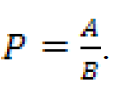
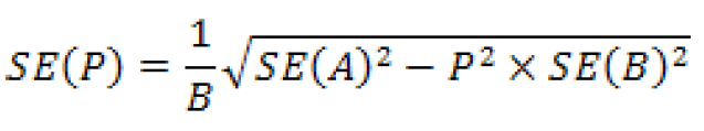
If the value under the square root sign is negative, then instead use
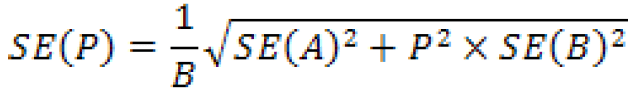
If P = 1 then use
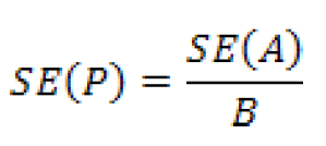
If Q = 100% x P (a percent instead of a proportion), then SE(Q) = 100% x SE(P).
- Means and Other Ratios
If the estimate is a ratio but the numerator is not a subset of the denominator, such as persons per household, per capita income, or percent change, then
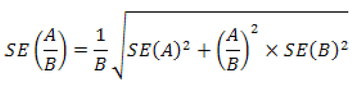
- Products
For a product of two estimates - for example if users want to estimate a proportion's numerator by multiplying the proportion by its denominator - the standard error can be approximated as
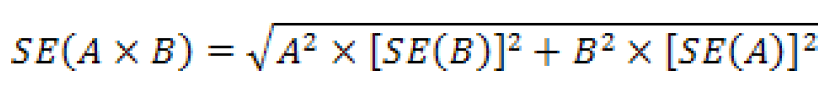
Users may combine these procedures for complicated estimates. For example, if the desired estimate is
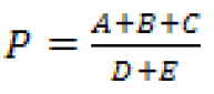 then SE(A+B+C) and SE(D+E) can be estimated first, and then those results used to calculate SE(P).
For examples of these formulas, please see any Accuracy of the Data document available under Data and Documentation on the ACS website http://www.census.gov/acs/www/.
Instructions for Statistical Testing
Once standard errors have been obtained, doing the statistical test to determine significance is not difficult. The determination of statistical significance takes into account the difference between the two estimates as well as the standard errors of both estimates. For two estimates, A and B, with standard errors SE(A) and SE(B), let
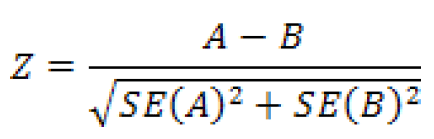
If Z < -1.645 or Z > 1.645, then the difference between A and B is significant at the 90 percent confidence level. Otherwise, the difference is not significant. This means that there is less than a 10 percent chance that the difference between these two estimates would be as large or larger by random chance alone.
This is the method used in determining statistical significance for the ACS Comparison Profiles published on AFF. Note that the user's determination of statistical significance may not match the results in the Comparison Profile for the same pair of estimates, because the significance tests for Comparison Profiles are made using unrounded standard errors. Standard errors obtained from the rounded margins of error or confidence bounds are unlikely to match the unrounded standard error, and so statistical tests may differ.
Users may choose to apply a confidence level different from 90 percent to their tests of statistical significance. For example, if Z < -1.96 or Z > 1.96, then the difference between A and B is significant at the 95 percent confidence level.
This method can be used for any types of estimates: counts, percentages, proportions, means, medians, etc. It can be used for comparing across years, or across surveys. If one of the estimates is a fixed value or comes from a source without sampling error (such as a count from the 2010 Census), use zero for the standard error for that estimate in the above equation for Z.
NOTE: Making comparisons between ACS single-year and multiyear estimates is very difficult, and is not advised.
In addition, using the rule of thumb of overlapping confidence intervals does not constitute a valid significance test and users are discouraged from using that method.
| Five-Group Classification | Fifteen-Group Classification | Examples |
| Science and Engineering | Computers, Mathematics and Statistics | Computer Science, Mathematics, General Statistics |
| Biological, Agricultural, and Environmental Sciences | Cellular and Molecular Biology, Soil Sciences, Natural Resource Management | |
| Physical and Related Sciences | Physics, Organic Chemistry, Astronomy | |
| Psychology | Psychology, Counseling, Child Psychology | |
| Social Sciences | Criminology, Sociology, Political Science | |
| Engineering | Chemical Engineering, Thermal Engineering, Electrical Engineering | |
| Multidisciplinary Studies | Nutritional Science, Cognitive Science, Behavioral Science | |
| Science and Engineering Related | Science and Engineering Related | Pre-Med, Physical Therapy, Mechanical Engineering Technology |
| Business | Business | Business Administration, Accounting, Human Resources Development |
| Education | Education | Early Childhood Education, Higher Education Administration, Special Education |
| Arts, Humanities, and Other | Literature and Languages | English, Foreign Language and Literature, Spanish |
| Liberal Arts and History | Philosophy, Theology, American History | |
| Visual and Performing Arts | Interior Design, Dance, Voice | |
| Communications | Mass Communications, Journalism, Public Relations | |
| Other | Public Administration, Pre-law, Kinesiology |
| Four Main Group Classifications | Thirty-Nine Subgroup Classifications |
| Spanish | Spanish or Spanish Creole Examples: Ladino, Pachuco |
French Examples: Cajun, Patois | |
French Creole Example: Haitian Creole | |
| Italian | |
Portuguese or Portuguese Creole Example: Papia Mentae | |
German Example: Luxembourgian | |
| Yiddish | |
Other West Germanic languages Examples: Dutch, Pennsylvania Dutch Afrikaans | |
Scandinavian languages Examples: Danish, Norwegian, Swedish | |
| Other Indo-European languages | Greek |
| Russian | |
| Polish | |
Serbo-Croatian Examples: Croatian, Serbian | |
Other Slavic languages Examples: Czech, Slovak, Ukrainian | |
| Armenian | |
| Persian | |
| Gujarati | |
| Hindi | |
| Urdu | |
Other Indic languages Examples: Bengali, Marathi, Punjabi, Romany | |
Other Indo-European languages Examples: Albanian, Gaelic, Lithuanian, Romanian | |
| Asian and Pacific Island languages | Chinese Examples: Cantonese, Formosan, Mandarin |
| Japanese | |
| Korean | |
| Mon-Khmer, Cambodian | |
| Hmong | |
| Thai | |
| Laotian | |
| Vietnamese | |
Other Asian languages Examples: Dravidian languages (Malayalam, Telugu, Tamil), Turkish | |
| Tagalog | |
Other Pacific Island languages Examples: Chamorro, Hawaiian, Ilocano, Indonesian, Samoan | |
| All other languages | Navajo |
Other Native North American languages Examples: Apache, Cherokee, Dakota, Pima, Yupik | |
| Hungarian | |
| Arabic | |
| Hebrew | |
African languages Examples: Amharic, Ibo, Yoruba, Bantu, Swahili, Somali | |
Other and unspecified languages Examples: Syriac, Finnish, Other languages of the Americas, not reported |
| Interview Month | Poverty Factors |
| January | 2.33074 |
| February | 2.3363 |
| March | 2.34179 |
| April | 2.34691 |
| May | 2.35138 |
| June | 2.3547 |
| July | 2.35795 |
| August | 2.3607 |
| September | 2.36401 |
| October | 2.36791 |
| November | 2.37214 |
| December | 2.37558 |
| Size of family unit | Related children under 18 years | ||||||||
| None | One | Two | Three | Four | Five | Six | Seven | Eight or more | |
| One person (unrelated individual) | N/A | N/A | N/A | N/A | N/A | N/A | N/A | N/A | N/A |
| Under 65 years | 5,019 | N/A | N/A | N/A | N/A | N/A | N/A | N/A | N/A |
| 65 years and over | 4,626 | N/A | N/A | N/A | N/A | N/A | N/A | N/A | N/A |
| Two persons | N/A | N/A | N/A | N/A | N/A | N/A | N/A | N/A | N/A |
| Householder under 65 years | 6,459 | 6,649 | N/A | N/A | N/A | N/A | N/A | N/A | N/A |
| Householder 65 years and over | 5,831 | 6,624 | N/A | N/A | N/A | N/A | N/A | N/A | N/A |
| Three persons | 7,546 | 7,765 | 7,772 | N/A | N/A | N/A | N/A | N/A | N/A |
| Four persons | 9,950 | 10,112 | 9,783 | 9,817 | N/A | N/A | N/A | N/A | N/A |
| Five persons | 11,999 | 12,173 | 11,801 | 11,512 | 11,336 | N/A | N/A | N/A | N/A |
| Six persons | 13,801 | 13,855 | 13,570 | 13,296 | 12,890 | 12,649 | N/A | N/A | N/A |
| Seven persons | 15,879 | 15,979 | 15,637 | 15,399 | 14,955 | 14,437 | 13,869 | N/A | N/A |
| Eight persons or more | 17,760 | 17,917 | 17,594 | 17,312 | 16,911 | 16,403 | 15,872 | 15,738 | N/A |
| Nine persons or more | 21,364 | 21,468 | 21,183 | 20,943 | 20,549 | 20,008 | 19,517 | 19,397 | 18,649 |
Source: U.S. Census Bureau
- White; Black or African American
- White; American Indian and Alaska Native
- White; Asian
- White; Native Hawaiian and Other Pacific Islander
- White; Some Other Race
- Black or African American; American Indian and Alaska Native
- Black or African American; Asian
- Black or African American; Native Hawaiian and Other Pacific Islander
- Black or African American; Some Other Race
- American Indian and Alaska Native; Asian
- American Indian and Alaska Native; Native Hawaiian and Other Pacific Islander
- American Indian and Alaska Native; Some other race
- Asian; Native Hawaiian and Other Pacific Islander
- Asian; Some Other Race
- Native Hawaiian and Other Pacific Islander; Some Other Race
- White; Black or African American; American Indian and Alaska Native
- White; Black or African American; Asian
- White; Black or African American; Native Hawaiian and Other Pacific Islander
- White; Black or African American; Some Other Race
- White; American Indian and Alaska Native; Asian
- White; American Indian and Alaska Native; Native Hawaiian and Other Pacific Islander
- White; American Indian and Alaska Native; Some Other Race
- White; Asian; Native Hawaiian and Other Pacific Islander
- White; Asian; Some Other Race
- White; Native Hawaiian and Other Pacific Islander; Some Other Race
- Black or African American; American Indian and Alaska Native; Asian
- Black or African American; American Indian and Alaska Native; Native Hawaiian and Other Pacific Islander
- Black or African American; American Indian and Alaska Native; Some Other Race
- Black or African American; Asian; Native Hawaiian and Other Pacific Islander
- Black or African American; Asian; Some Other Race
- Black or African American; Native Hawaiian and Other Pacific Islander; Some Other Race
- American Indian and Alaska Native; Asian; Native Hawaiian and Other Pacific Islander
- American Indian and Alaska Native; Asian; Some Other Race
- American Indian and Alaska Native; Native Hawaiian and Other Pacific Islander; Some Other Race
- Asian; Native Hawaiian and Other Pacific Islander; Some Other Race
- White; Black or African American; American Indian and Alaska Native; Asian
- White; Black or African American; American Indian and Alaska Native; Native Hawaiian and Other Pacific Islander
- White; Black or African American; American Indian and Alaska Native; Some Other Race
- White; Black or African American; Asian; Native Hawaiian and Other Pacific Islander
- White; Black or African American; Asian; Some Other Race
- White; Black or African American; Native Hawaiian and Other Pacific Islander; Some Other Race
- White; American Indian and Alaska Native; Asian; Native Hawaiian and Other Pacific Islander
- White; American Indian and Alaska Native; Asian; Some Other Race
- White; American Indian and Alaska Native; Native Hawaiian and Other Pacific Islander; Some other race
- White; Asian; Native Hawaiian and Other Pacific Islander; Some Other Race
- Black or African American; American Indian and Alaska Native; Asian; Native Hawaiian and Other Pacific Islander
- Black or African American; American Indian and Alaska Native; Asian; Some Other Race
- Black or African American; American Indian and Alaska Native; Native Hawaiian and Other Pacific Islander; Some Other Race
- Black or African American; Asian; Native Hawaiian and Other Pacific Islander; Some Other Race
- American Indian and Alaska Native; Asian; Native Hawaiian and Other Pacific Islander; Some Other Race
- White; Black or African American; American Indian and Alaska Native; Asian; Native Hawaiian and Other Pacific Islander
- White; Black or African American; American Indian and Alaska Native; Asian; Some Other Race
- White; Black or African American; American Indian and Alaska Native; Native Hawaiian and Other Pacific Islander; Some Other Race
- White; Black or African American; Asian; Native Hawaiian and Other Pacific Islander; Some Other Race
- White; American Indian and Alaska Native; Asian; Native Hawaiian and Other Pacific Islander; Some Other Race
- Black or African American; American Indian and Alaska Native; Asian; Native Hawaiian and Other Pacific Islander; Some Other Race
- White; Black or African American; American Indian and Alaska Native; Asian; Native Hawaiian and Other Pacific Islander; Some Other Race
| Standard Distribution for Median Age: |
| [116 data cells] |
| Under 1 year |
| 1 year |
| 2 years |
| 3 years |
| 4 years |
| 5 years |
| . |
| . |
| . |
| 112 years |
| 113 years |
| 114 years |
| 115 years and over |
| Standard Distribution for Median Agricultural Crop Sales: |
| [5 data cells] |
| Less than $1,000 |
| $1,000 to $2,499 |
| $2,500 to $4,999 |
| $5,000 to $9,999 |
| $10,000 or more |
| Standard Distribution for Median Bedrooms: |
| [9 data cells] |
| No bedroom |
| 1 bedroom |
| 2 bedrooms |
| 3 bedrooms |
| 4 bedrooms |
| 5 bedrooms |
| 6 bedrooms |
| 7 bedrooms |
| 8 or more bedrooms |
| Standard Distribution for Median Condominium Fees: |
| [15 data cells] |
| Less than $50 |
| $50 to $99 |
| $100 to $199 |
| $200 to $299 |
| $300 to $399 |
| $400 to $499 |
| $500 to $599 |
| $600 to $699 |
| $700 to $799 |
| $800 to $899 |
| $900 to $999 |
| $1,000 to $1,249 |
| $1,250 to $1,499 |
| $1,500 to $1,749 |
| $1,750 or more |
| Standard Distribution for Median Contract Rent/Quartile Contract Rent/Rent Asked/Gross Rent: |
| [23 data cells] |
| Less than $100 |
| $100 to $149 |
| $150 to $199 |
| $200 to $249 |
| $250 to $299 |
| $300 to $349 |
| $350 to $399 |
| $400 to $449 |
| $450 to $499 |
| $500 to $549 |
| $550 to $599 |
| $600 to $649 |
| $650 to $699 |
| $700 to $749 |
| $750 to $799 |
| $800 to $899 |
| $900 to $999 |
| $1,000 to $1,249 |
| $1,250 to $1,499 |
| $1,500 to $1,999 |
| $2,000 to $2,499 |
| $2,500 to $2,999 |
| $3,000 or more |
| Standard Distribution for Duration of Current Marriage: |
| [101 data cells] |
| Under 1 year |
| 1 year |
| 2 years |
| 3 years |
| 4 years |
| 5 years |
| . |
| . |
| . |
| 97 years |
| 98 years |
| 99 years |
| 100 years and over |
| Standard Distribution for Median Earnings and Median Income (Individuals): |
| [101 data cells] |
| Less than $2,500 |
| $2,500 to $4,999 |
| $5,000 to $7,499 |
| $7,500 to $9,999 |
| $10,000 to $12,499 |
| $12,500 to $14,999 |
| $15,000 to $17,499 |
| $17,500 to $19,999 |
| $20,000 to $22,499 |
| $22,500 to $24,999 |
| $25,000 to $27,499 |
| $27,500 to $29,999 |
| $30,000 to $32,499 |
| $32,500 to $34,999 |
| $35,000 to $37,499 |
| $37,500 to $39,999 |
| $40,000 to $42,499 |
| $42,500 to $44,999 |
| $45,000 to $47,499 |
| $47,500 to $49,999 |
| $50,000 to $52,499 |
| $52,500 to $54,999 |
| $55,000 to $57,499 |
| $57,500 to $59,999 |
| $60,000 to $62,499 |
| $62,500 to $64,999 |
| $65,000 to $67,499 |
| $67,500 to $69,999 |
| $70,000 to $72,499 |
| $72,500 to $74,999 |
| $75,000 to $77,499 |
| $77,500 to $79,999 |
| $80,000 to $82,499 |
| $82,500 to $84,999 |
| $85,000 to $87,499 |
| $87,500 to $89,999 |
| $90,000 to $92,499 |
| $92,500 to $94,999 |
| $95,000 to $97,499 |
| $97,500 to $99,999 |
| $100,000 to $102,499 |
| $102,500 to $104,999 |
| $105,000 to $107,499 |
| $107,500 to $109,999 |
| $110,000 to $112,499 |
| $112,500 to $114,999 |
| $115,000 to $117,499 |
| $117,500 to $119,999 |
| $120,000 to $122,499 |
| $122,500 to $124,999 |
| $125,000 to $127,499 |
| $127,500 to $129,999 |
| $130,000 to $132,499 |
| $132,500 to $134,999 |
| $135,000 to $137,499 |
| $137,500 to $139,999 |
| $140,000 to $142,499 |
| $142,500 to $144,999 |
| $145,000 to $147,499 |
| $147,500 to $149,999 |
| $150,000 to $152,499 |
| $152,500 to $154,999 |
| $155,000 to $157,499 |
| $157,500 to $159,999 |
| $160,000 to $162,499 |
| $162,500 to $164,999 |
| $165,000 to $167,499 |
| $167,500 to $169,999 |
| $170,000 to $172,499 |
| $172,500 to $174,999 |
| $175,000 to $177,499 |
| $177,500 to $179,999 |
| $180,000 to $182,499 |
| $182,500 to $184,999 |
| $185,000 to $187,499 |
| $187,500 to $189,999 |
| $190,000 to $192,499 |
| $192,500 to $194,999 |
| $195,000 to $197,499 |
| $197,500 to $199,999 |
| $200,000 to $202,499 |
| $202,500 to $204,999 |
| $205,000 to $207,499 |
| $207,500 to $209,999 |
| $210,000 to $212,499 |
| $212,500 to $214,999 |
| $215,000 to $217,499 |
| $217,500 to $219,999 |
| $220,000 to $222,499 |
| $222,500 to $224,999 |
| $225,000 to $227,499 |
| $227,500 to $229,999 |
| $230,000 to $232,499 |
| $232,500 to $234,999 |
| $235,000 to $237,499 |
| $237,500 to $239,999 |
| $240,000 to $242,499 |
| $242,500 to $244,999 |
| $245,000 to $247,499 |
| $247,500 to $249,999 |
| $250,000 or more |
| Standard Distribution for Median Fire, Hazard, and Flood Insurance: |
| [19 data cells] |
| $0 |
| $1 to $49 |
| $50 to $99 |
| $100 to $149 |
| $150 to $199 |
| $200 to $249 |
| $250 to $299 |
| $300 to $349 |
| $350 to $399 |
| $400 to $449 |
| $450 to $499 |
| $500 to $599 |
| $600 to $699 |
| $700 to $799 |
| $800 to $899 |
| $900 to $999 |
| $1,000 to $1,499 |
| $1,500 to $1,999 |
| $2,000 or more |
| Standard Distribution for Median Gross Rent as a Percentage of Household Income: |
| [13 data cells] |
| Less than 10.0 percent |
| 10.0 to 14.9 percent |
| 15.0 to 19.9 percent |
| 20.0 to 24.9 percent |
| 25.0 to 29.9 percent |
| 30.0 to 34.9 percent |
| 35.0 to 39.9 percent |
| 40.0 to 49.9 percent |
| 50.0 to 59.9 percent |
| 60.0 to 69.9 percent |
| 70.0 to 79.9 percent |
| 80.0 to 89.9 percent |
| 90.0 percent or more |
| Standard Distribution for Median Income in the Past 12 Months (Household/Family/Nonfamily Household): |
| [101 data cells] |
| Less than $2,500 |
| $2,500 to $4,999 |
| $5,000 to $7,499 |
| $7,500 to $9,999 |
| $10,000 to $12,499 |
| $12,500 to $14,999 |
| $15,000 to $17,499 |
| $17,500 to $19,999 |
| $20,000 to $22,499 |
| $22,500 to $24,999 |
| $25,000 to $27,499 |
| $27,500 to $29,999 |
| $30,000 to $32,499 |
| $32,500 to $34,999 |
| $35,000 to $37,499 |
| $37,500 to $39,999 |
| $40,000 to $42,499 |
| $42,500 to $44,999 |
| $45,000 to $47,499 |
| $47,500 to $49,999 |
| $50,000 to $52,499 |
| $52,500 to $54,999 |
| $55,000 to $57,499 |
| $57,500 to $59,999 |
| $60,000 to $62,499 |
| $62,500 to $64,999 |
| $65,000 to $67,499 |
| $67,500 to $69,999 |
| $70,000 to $72,499 |
| $72,500 to $74,999 |
| $75,000 to $77,499 |
| $77,500 to $79,999 |
| $80,000 to $82,499 |
| $82,500 to $84,999 |
| $85,000 to $87,499 |
| $87,500 to $89,999 |
| $90,000 to $92,499 |
| $92,500 to $94,999 |
| $95,000 to $97,499 |
| $97,500 to $99,999 |
| $100,000 to $102,499 |
| $102,500 to $104,999 |
| $105,000 to $107,499 |
| $107,500 to $109,999 |
| $110,000 to $112,499 |
| $112,500 to $114,999 |
| $115,000 to $117,499 |
| $117,500 to $119,999 |
| $120,000 to $122,499 |
| $122,500 to $124,999 |
| $125,000 to $127,499 |
| $127,500 to $129,999 |
| $130,000 to $132,499 |
| $132,500 to $134,999 |
| $135,000 to $137,499 |
| $137,500 to $139,999 |
| $140,000 to $142,499 |
| $142,500 to $144,999 |
| $145,000 to $147,499 |
| $147,500 to $149,999 |
| $150,000 to $152,499 |
| $152,500 to $154,999 |
| $155,000 to $157,499 |
| $157,500 to $159,999 |
| $160,000 to $162,499 |
| $162,500 to $164,999 |
| $165,000 to $167,499 |
| $167,500 to $169,999 |
| $170,000 to $172,499 |
| $172,500 to $174,999 |
| $175,000 to $177,499 |
| $177,500 to $179,999 |
| $180,000 to $182,499 |
| $182,500 to $184,999 |
| $185,000 to $187,499 |
| $187,500 to $189,999 |
| $190,000 to $192,499 |
| $192,500 to $194,999 |
| $195,000 to $197,499 |
| $197,500 to $199,999 |
| $200,000 to $202,499 |
| $202,500 to $204,999 |
| $205,000 to $207,499 |
| $207,500 to $209,999 |
| $210,000 to $212,499 |
| $212,500 to $214,999 |
| $215,000 to $217,499 |
| $217,500 to $219,999 |
| $220,000 to $222,499 |
| $222,500 to $224,999 |
| $225,000 to $227,499 |
| $227,500 to $229,999 |
| $230,000 to $232,499 |
| $232,500 to $234,999 |
| $235,000 to $237,499 |
| $237,500 to $239,999 |
| $240,000 to $242,499 |
| $242,500 to $244,999 |
| $245,000 to $247,499 |
| $247,500 to $249,999 |
| $250,000 or more |
| Standard Distribution for Median Monthly Housing Costs: |
| [30 cells] |
| Less than $100 |
| $100 to $149 |
| $150 to $199 |
| $200 to $249 |
| $250 to $299 |
| $300 to $349 |
| $350 to $399 |
| $400 to $449 |
| $450 to $499 |
| $500 to $549 |
| $550 to $599 |
| $600 to $649 |
| $650 to $699 |
| $700 to $749 |
| $750 to $799 |
| $800 to $899 |
| $900 to $999 |
| $1,000 to $1,249 |
| $1,250 to $1,499 |
| $1,500 to $1,749 |
| $1,750 to $1,999 |
| $2,000 to $2,499 |
| $2,500 to $2,999 |
| $3,000 to $3,499 |
| $3,500 to $3,999 |
| $4,000 to $4,499 |
| $4,500 to $4,999 |
| $5,000 to $5,499 |
| $5,500 to $5,999 |
| $6,000 or more |
| Standard Distribution for Median Real Estate Taxes Paid: |
| [14 data cells] |
| Less than $200 |
| $200 to $299 |
| $300 to $399 |
| $400 to $599 |
| $600 to $799 |
| $800 to $999 |
| $1,000 to $1,499 |
| $1,500 to $1,999 |
| $2,000 to $2,999 |
| $3,000 to $3,999 |
| $4,000 to $4,999 |
| $5,000 to $7,499 |
| $7,500 to $9,999 |
| $10,000 or more |
| Standard Distribution for Median Rooms: |
| [14 data cells] |
| 1 room |
| 2 rooms |
| 3 rooms |
| 4 rooms |
| 5 rooms |
| 6 rooms |
| 7 rooms |
| 8 rooms |
| 9 rooms |
| 10 rooms |
| 11 rooms |
| 12 rooms |
| 13 rooms |
| 14 or more rooms |
| Standard Distribution for Median Selected Monthly Owner Costs/Median Selected Monthly Owner Costs by Mortgage Status (With a Mortgage): |
| [23 data cells] |
| Less than $100 |
| $100 to $199 |
| $200 to $299 |
| $300 to $399 |
| $400 to $499 |
| $500 to $599 |
| $600 to $699 |
| $700 to $799 |
| $800 to $899 |
| $900 to $999 |
| $1,000 to $1,249 |
| $1,250 to $1,499 |
| $1,500 to $1,749 |
| $1,750 to $1,999 |
| $2,000 to $2,499 |
| $2,500 to $2,999 |
| $3,000 to $3,499 |
| $3,500 to $3,999 |
| $4,000 to $4,499 |
| $4,500 to $4,999 |
| $5,000 to $5,499 |
| $5,500 to $5,999 |
| $6,000 or more |
| Standard Distribution for Median Selected Monthly Owner Costs by Mortgage Status (Without a Mortgage): |
| [17 data cells] |
| Less than $100 |
| $100 to $149 |
| $150 to $199 |
| $200 to $249 |
| $250 to $299 |
| $300 to $349 |
| $350 to $399 |
| $400 to $499 |
| $500 to $599 |
| $600 to $699 |
| $700 to $799 |
| $800 to $899 |
| $900 to $999 |
| $1,000 to $1,249 |
| $1,250 to $1,499 |
| $1,500 to $1,999 |
| $2,000 or more |
| Standard Distribution for Median Selected Monthly Owner Costs as a Percentage of Household Income by Mortgage Status: |
| [13 data cells] |
| Less than 10.0 percent |
| 10.0 to 14.9 percent |
| 15.0 to 19.9 percent |
| 20.0 to 24.9 percent |
| 25.0 to 29.9 percent |
| 30.0 to 34.9 percent |
| 35.0 to 39.9 percent |
| 40.0 to 49.9 percent |
| 50.0 to 59.9 percent |
| 60.0 to 69.9 percent |
| 70.0 to 79.9 percent |
| 80.0 to 89.9 percent |
| 90.0 percent or more |
| Standard Distribution for Median Total Mortgage Payment: |
| [21 data cells] |
| Less than $100 |
| $100 to $199 |
| $200 to $299 |
| $300 to $399 |
| $400 to $499 |
| $500 to $599 |
| $600 to $699 |
| $700 to $799 |
| $800 to $899 |
| $900 to $999 |
| $1,000 to $1,249 |
| $1,250 to $1,499 |
| $1,500 to $1,749 |
| $1,750 to $1,999 |
| $2,000 to $2,499 |
| $2,500 to $2,999 |
| $3,000 to $3,499 |
| $3,500 to $3,999 |
| $4,000 to $4,499 |
| $4,500 to $4,999 |
| $5,000 or more |
| Standard Distribution for Median Usual Hours Worked Per Week Worked in the Past 12 Months: |
| [9 data cells] |
| Usually worked 50 to 99 hours per week |
| Usually worked 45 to 49 hours per week |
| Usually worked 41 to 44 hours per week |
| Usually worked 40 hours per week |
| Usually worked 35 to 39 hours per week |
| Usually worked 30 to 34 hours per week |
| Usually worked 25 to 29 hours per week |
| Usually worked 15 to 24 hours per week |
| Usually worked 1 to 14 hours per week |
| Standard Distribution for Median Value/Quartile Value/Price Asked: |
| [24 data cells] |
| Less than $10,000 |
| $10,000 to $14,999 |
| $15,000 to $19,999 |
| $20,000 to $24,999 |
| $25,000 to $29,999 |
| $30,000 to $34,999 |
| $35,000 to $39,999 |
| $40,000 to $49,999 |
| $50,000 to $59,999 |
| $60,000 to $69,999 |
| $70,000 to $79,999 |
| $80,000 to $89,999 |
| $90,000 to $99,999 |
| $100,000 to $124,999 |
| $125,000 to $149,999 |
| $150,000 to $174,999 |
| $175,000 to $199,999 |
| $200,000 to $249,999 |
| $250,000 to $299,999 |
| $300,000 to $399,999 |
| $400,000 to $499,999 |
| $500,000 to $749,999 |
| $750,000 to $999,999 |
| $1,000,000 or more |
| Standard Distribution for Median Vehicles Available: |
| [6 data cells] |
| No vehicle available |
| 1 vehicle available |
| 2 vehicles available |
| 3 vehicles available |
| 4 vehicles available |
| 5 or more vehicles available |
| Standard Distribution for Median Year Householder Moved Into Unit: |
| [16 data cells] |
| Moved in 2011 |
| Moved in 2010 |
| Moved in 2009 |
| Moved in 2008 |
| Moved in 2007 |
| Moved in 2006 |
| Moved in 2005 |
| Moved in 2004 |
| Moved in 2003 |
| Moved in 2002 |
| Moved in 2001 |
| Moved in 2000 |
| Moved in 1990 to 1999 |
| Moved in 1980 to 1989 |
| Moved in 1970 to 1979 |
| Moved in 1969 or earlier |
| Standard Distribution for Median Year Structure Built: |
| [19 data cells] |
| Built in 2011 |
| Built in 2010 |
| Built in 2009 |
| Built in 2008 |
| Built in 2007 |
| Built in 2006 |
| Built in 2005 |
| Built in 2004 |
| Built in 2003 |
| Built in 2002 |
| Built in 2001 |
| Built in 2000 |
| Built 1990 to 1999 |
| Built 1980 to 1989 |
| Built 1970 to 1979 |
| Built 1960 to 1969 |
| Built 1950 to 1959 |
| Built 1940 to 1949 |
| Built 1939 or earlier |
Additional information on the design and methodology of the ACS, including data collection and processing, can be found at: http://www.census.gov/acs/www/methodology/methodology_main/.
The 2012 Accuracy of the Data from the Puerto Rico Community Survey can be found at
http://www.census.gov/acs/www/Downloads/data_documentation/Accuracy/PRCS_Accuracy_of_Data_2012.pdf.
The ACS employs three modes of data collection:
- Mailout/Mailback
- Computer Assisted Telephone Interview (CATI)
- Computer Assisted Personal Interview (CAPI)
With the exception of addresses in Remote Alaska, the general timing of data collection is:
Month 1: Addresses in sample that are determined to be mailable are sent a questionnaire via
the U.S. Postal Service.
Month 2: All mail non-responding addresses with an available phone number are sent to CATI.
Month 3: A sample of mail non-responses without a phone number, CATI non-responses, and unmailable addresses are selected and sent to CAPI.
Note that mail responses are accepted during all three months of data collection.
All Remote Alaska addresses that are in sample are assigned to one of two data collection periods, January-April, or September-December and are all sent to the CAPI mode of data collection.1 Data for these addresses are collected using CAPI only and up to four months are given to complete the interviews in Remote Alaska for each data collection period.
1 Prior to the 2011 sample year, all remote Alaska sample cases were subsampled for CAPI at a rate of 2-in-3.
Field representatives have several options available to them for data collection. These include completing the questionnaire while speaking to the resident in person or over the telephone, conducting a personal interview with a proxy, such as a relative or guardian, or leaving paper questionnaires for residents to complete for themselves and then pick them up later. This last option is used for data collection in Federal prisons.
- Soup kitchens
- Domestic violence shelters
- Regularly scheduled mobile food vans
- Targeted non-sheltered outdoor locations
- Maritime/merchant vessels
- Living quarters for victims of natural disasters
The Main sample is selected during the summer preceding the sample year. Approximately 99 percent of the sample is selected at this time. Each address in sample is randomly assigned to one of the 12 months of the sample year. Supplemental sampling occurs in January/February of the sample year and accounts for approximately 1 percent of the overall first-phase sample. The Supplemental sample is allocated to the last six months of the sample year. A sub-sample of non-responding addresses and of any addresses deemed unmailable is selected for the CAPI data collection mode2.
Several steps used to select the first-phase sample are common to both Main and Supplemental sampling. The descriptions of the steps included in the first-phase sample selection below indicate which are common to both and which are unique to either Main or Supplemental sampling.
1. First-phase Sample Selection
- First-stage sampling (performed during both Main and Supplemental sampling) - First stage sampling defines the universe for the second stage of sampling through two steps. First, all addresses that were in a first-phase sample within the past four years are excluded from eligibility. This ensures that no address is in sample more than once in any five-year period. The second step is to select a 20 percent systematic sample of "new" units, i.e. those units that have never appeared on a previous MAF extract. Each new address is systematically assigned to either the current year or to one of four back- samples. This procedure maintains five equal partitions (samples) of the universe.
- Assignment of blocks to a second-stage sampling stratum (performed during Main sampling only) - Second-stage sampling uses 16 sampling strata in the U.S3. The stratum level rates used in second-stage sampling account for the first-stage selection probabilities. These rates are applied at a block level to addresses in the U.S. by calculating a measure of size for each of the following geographic entities:
- Counties
- Places
- School Districts (elementary, secondary, and unified)
- American Indian Areas
- Tribal Subdivisions
- Alaska Native Village Statistical Areas
- Hawaiian Homelands
- Minor Civil Divisions - in Connecticut, Maine, Massachusetts, Michigan, Minnesota, New Hampshire, New Jersey, New York, Pennsylvania, Rhode Island, Vermont, and Wisconsin (these are the states where MCDs are active, functioning governmental units)
- Census Designated Places - in Hawaii only
The measure of size for all areas except American Indian Areas, Tribal Subdivisions, and Alaska Native Village Statistical Areas is an estimate of the number of occupied HUs in the area. This is calculated by multiplying the number of ACS addresses by an estimated occupancy rate at the block level. A measure of size for each Census Tract is also calculated in the same manner.
For American Indian, Tribal Subdivisions, and Alaska Native Village Statistical Areas, the measure of size is the estimated number of occupied HUs multiplied by the proportion of people reporting American Indian or Alaska Native (alone or in combination) in the 2010 Census.
Each block is then assigned the smallest measure of size from the set of all entities of which it is a part. The 2012 second-stage sampling strata and the overall first-phase sampling rates are shown in Table 1 below. The sample rates represent the actual percent in sample that was delivered for the 2012 sample year.
- Calculation of the second-stage sampling rates (performed during Main sampling only) - The overall first-phase sampling rates given in Table 1 are calculated using the distribution of ACS valid addresses by second-stage sampling stratum in such a way as to yield an overall target sample size for the year of 3,540,000 in the U.S. These rates also account for expected growth of the HU inventory between Main and Supplemental of roughly 1 percent. The first-phase rates are adjusted for the first-stage sample to yield the second-stage selection probabilities4.
- Second-stage sample selection (performed in Main and Supplemental) - After each block is assigned to a second-stage sampling stratum, a systematic sample of addresses is selected from the second-stage universe (first-stage sample) within each county and county equivalent.
- Sample Month Assignment (performed in Main and Supplemental) - After the second stage of sampling, all sample addresses are randomly assigned to a sample month. Addresses selected during Main sampling are allocated to each of the 12 months. Addresses selected during Supplemental sampling are assigned to the months of May- December.
Table 1. First-phase Sampling Rate Categories for the United States
| Sampling Stratum | Type of Area | Rate Definitions | 2012 Sampling Rate |
| 1 | 0 < MOS1 ≤ 200 | 15% | 15.00% |
| 2 | 200 < MOS ≤ 400 | 10% | 10.00% |
| 3 | 400 < MOS ≤ 800 | 7% | 7.00% |
| 4 | 800 < MOS ≤ 1,200 | 2.8 × BR | 4.40% |
| 5 | 0 < TRACTMOS2 ≤ 400 | 3.5 × BR | 5.55% |
| 6 | 0 < TRACTMOS ≤ 400 H.R.3 | 0.92 × 3.5 × BR | 5.06% |
| 7 | 400 < TRACTMOS ≤ 1,000 | 2.8 × BR | 4.40% |
| 8 | 400 < TRACTMOS ≤ 1,000 H.R. | 0.92 × 2.8 × BR | 4.04% |
| 9 | 1,000 < TRACTMOS ≤ 2,000 | 1.7 × BR | 2.67% |
| 10 | 1,000 < TRACTMOS ≤ 2,000 H.R. | 0.92 × 1.7 × BR | 2.46% |
| 11 | 2,000 < TRACTMOS ≤ 4,000 | BR4 | 1.57% |
| 12 | 2,000 < TRACTMOS ≤ 4,000 H.R. | 0.92 × BR | 1.44% |
| 13 | 4,000 < TRACTMOS ≤ 6,000 | 0.6 × BR | 0.94% |
| 14 | 4,000 < TRACTMOS ≤ 6,000 H.R. | 0.92 × 0.6 × BR | 0.87% |
| 15 | 6,000 < TRACTMOS | 0.35 × BR | 0.55% |
| 16 | 6,000 < TRACTMOS H.R. | 0.92 × 0.35 × BR | 0.51% |
| 1MOS = measure of size (estimated number occupied housing units) of the smallest governmental entity | |||
| 2TRACTMOS = the measure of size (MOS) at the Census Tract level | |||
| 3H.R. = areas where predicted levels of completed mail and CATI interviews are > 60% | |||
| 4BR = base sampling rate | |||
| 5NA = not applicable | |||
2. Second-phase Sample Selection - Subsampling the Unmailable and Non-Responding Addresses
Most addresses determined to be unmailable are subsampled for the CAPI phase of data collection at a rate of 2-in-3. Unmailable addresses, which include Remote Alaska addresses, do not go to the CATI phase of data collection. Subsequent to CATI, all addresses for which no response has been obtained prior to CAPI are subsampled based on the expected rate of completed interviews at the tract level using the rates shown in Table 2.
Table 2. Second-Phase (CAPI) Subsampling Rates for the United States
| Address and Tract Characteristics | CAPI Subsampling Rate |
| United States | |
| Addresses in Remote Alaska1 | Take all (100%) |
| Addresses in Hawaiian Homelands, Alaska Native Village Statistical areas and a subset of American Indian areas1 | Take all (100%) |
| Unmailable addresses that are not in the previous two categories | 66.70% |
| Mailable addresses in tracts with predicted levels of completed mail and CATI interviews prior to CAPI subsampling between 0% and less than 36% | 50.00% |
| Mailable addresses in tracts with predicted levels of completed mail and CATI interviews prior to CAPI subsampling greater than 35% and less than 51% | 40.00% |
| Mailable addresses in other tracts | 33.30% |
| 1The full CAPI follow-up procedure for these two categories is new to the ACS sample design. | |
2Beginning with the August, 2011 CAPI sample all non-mailable and non-responding addresses in the following areas are now sent to CAPI: all Hawaiian Homelands, all Alaska Native Village Statistical areas, American Indian areas with an estimated proportion of American Indian population ≥ 10%.
3Beginning with the 2011 sample the ACS implemented a change to the stratification, increasing the number of sampling strata and changing how the sampling rates are defined. Prior to 2011 there were seven strata, there are now 16 sampling strata. Table 1 gives a summary of these strata and the rates.
4The annual target sample size for the ACS was increased to the 3.54 million level beginning with the June, 2011 panel. Therefore, the U.S sample size increased from roughly 242,000 per month to 295,000 per month starting with the June, 2011 mail-out. The final 2011 sample was 3,272,520. The annual target sample size remains at 3.54 million.
1. First-phase Sample Selection for Small GQ Stratum
- First-stage sampling - Small GQs are only eligible to be selected for the ACS once every five years. To accomplish this, the first stage sampling procedure systematically assigned all small GQs to one of five partitions of the universe. Each partition was assigned to a particular year (2012-2016) and the one assigned to 2012 became the first stage sample. In future years, each new GQ will be systematically assigned to one of the five samples. These samples are rotated over five year periods and become the universe for selecting the second stage sample.
- Second-stage sampling - During the second stage, GQs are selected from the first stage sample in a systematic sample of 1-in-x where x is dependent upon the state's target sampling rate. Since the first stage sample is one fifth of the universe, x can be calculated as x = (1 /5) x (1 / rate) where rate is the state's target sampling rate. For example, suppose a state had a target sampling rate of 2.5%. The systematic sample would then be 1-in-8 since (1 / 5) x (1 / 0.025) = 8. Regardless of their actual size, all GQs in the small stratum have the same probability of selection.
Unlike housing unit address sampling and the small GQ sample selection, the large GQ sampling procedure has no first-stage in which sampling units are randomly assigned to one of five years. All large GQs are eligible for sampling each year. The large GQ samples are selected using a two-phase design.
- First-phase Sampling
All GQs in this stratum are eligible for sampling every year, regardless of their sample status in previous years. For large GQs, hits can be selected multiple times in the sample year. For most GQ types, the hits are randomly assigned throughout the year. Some GQs may have multiple hits with the same sample date if more than 12 hits are selected from the GQ. In these cases, the person sample within that month is unduplicated. The following table summarizes the 2012 state target sampling rates for the U.S.
Table 3. 2012 State Targeted Sampling Rates for the U.S.
| Alabama | 2.17% | Iowa | 2.40% | New York | 2.29% |
| Alaska | 4.19% | Kentucky | 2.38% | North Dakota | 4.49% |
| Arizona | 2.05% | Louisiana | 2.60% | Oregon, Puerto Rico | 2.50% |
| Arkansas, Illinois | 2.21% | Maine | 3.09% | Pennsylvania | 2.53% |
| California | 2.49% | Massachusetts | 2.22% | Rhode Island | 2.63% |
| Colorado | 2.33% | Michigan | 2.79% | South Carolina | 2.26% |
| Connecticut | 2.37% | Minnesota, Wisconsin | 2.47% | South Dakota | 3.51% |
| Delaware | 5.00% | Mississippi | 2.32% | Tennessee | 2.30% |
| District of Columbia, New Mexico | 2.77% | Missouri | 2.25% | Texas | 2.16% |
| Florida, North Carolina | 2.34% | Montana | 3.96% | Vermont | 4.39% |
| Georgia, Kansas, Maryland, Ohio, Oklahoma | 2.39% | Nebraska | 2.46% | Virginia | 2.20% |
| Hawaii, Utah | 3.00% | Nevada | 3.63% | Washington | 2.45% |
| Idaho | 4.13% | New Hampshire | 2.90% | West Virginia | 2.31% |
| Indiana | 2.35% | New Jersey | 2.72% | Wyoming | 6.97% |
3. Sample Month Assignment
In order to assign each hit to a panel month, all of the GQ samples from a state are combined and sorted by small/large stratum and second-phase order of selection. Consecutive samples are assigned to the twelve panel months in a predetermined order, starting with a randomly determined month, except for Federal prisons and remote Alaska. Remote Alaska GQs are assigned to January and September based on where the GQ is located. Correctional facilities have their sample clustered. All Federal prisons hits are assigned to the September panel. In non-Federal correctional facilities, all hits for a given GQ are assigned to the same panel month. However, unlike Federal prisons, the hits in state and local correctional facilities are assigned to randomly selected panels spread throughout the year.
4. Second Phase Sample: Selection of Persons in Small and Large GQs
Small GQs in the second phase sampling are "take all," i.e., every person in the selected GQ is eligible to receive a questionnaire. If the actual number of persons in the GQ exceeds 15, a field subsampling operation is performed to reduce the total number of sample persons interviewed at the GQ to 10. If the actual number of people is 15 or less, all people in the GQ will receive the questionnaire.
For each hit in the large GQs, the automated instrument uses the population count at the time of the visit and selects a subsample of 10 people from the roster. The people in this subsample receive the questionnaire.
The weighting is conducted in two main operations: a group quarters person weighting operation which assigns weights to persons in group quarters, and a household person weighting operation which assigns weights both to housing units and to persons within housing units. The group quarters person weighting is conducted first and the household person weighting second. The household person weighting is dependent on the group quarters person weighting because estimates for total population which include both group quarters and household population are controlled to the Census Bureau's official 2012 total resident population estimates.
- The primary objective was to establish representation of county by major GQ type group in the tabulations for each combination that exists on the ACS GQ sample frame. The seven major GQ type groups are defined by the Population Estimates Program and are given in Table 4.
- A secondary objective was to establish representation of tract by major GQ type group for each combination that exists on the ACS GQ sample frame.
Table 4: Population Estimates Program Major GQ Type Groups
| Major GQ Type Group | Definition | Institutional / Non-Institutional |
| 1 | Correctional Institutions | Institutional |
| 2 | Juvenile Detention Facilities | Institutional |
| 3 | Nursing Homes | Institutional |
| 4 | Other Long-Term Care Facilities | Institutional |
| 5 | College Dormitories | Non-Institutional |
| 6 | Military Facilities | Non-Institutional |
| 7 | Other Non-Institutional Facilities | Non-Institutional |
For all not-in-sample GQ facilities with an expected population of 16 or more persons (large facilities), we imputed a number of GQ persons equal to 2.5% of the expected population. For those GQ facilities with an expected population of fewer than 16 persons (small facilities), we selected a random sample of GQ facilities as needed to accomplish the two objectives given above. For those selected small GQ facilities, we imputed a number of GQ persons equal to 20% of the facility's expected population.
Interviewed GQ person records were then sampled at random to be imputed into the selected not-in-sample GQ facilities. An expanding search algorithm searched for donors within the same specific type of GQ facility and the same county. If that failed, the search included all GQ facilities of the same major GQ type group. If that still failed, the search expanded to a specific type within a larger geography, then a major GQ type group within that geography, and so on until suitable donors were found.
The weighting procedure made no distinction between sampled and imputed GQ person records. The initial weights of person records in the large GQ facilities equaled the observed or expected population of the GQ facility divided by the number of person records. The initial weights of person records in small GQ facilities equaled the observed or expected population of the GQ facility divided by the number of records, multiplied by the inverse of the fraction represented on the frame of the small GQ facilities of that tract by major GQ type group combination. As was done in previous years' weighting, we controlled the final weights to an independent set of GQ population estimates produced by the Population Estimates Program for each state by each of the seven major GQ type groups.
Lastly, the final GQ person weight was rounded to an integer. Rounding was performed so that the sum of the rounded weights were within one person of the sum of the unrounded weights for any of the groups listed below:
Major GQ Type Group
Major GQ Type Group x County
Weighting areas were built from collections of whole counties. 2010 Census data and 2007-2011 ACS 5-year data were used to group counties of similar demographic and social characteristics. The characteristics considered in the formation included:
- Percent in poverty (the only characteristic using ACS 5-year data)
- Percent renting
- Density of housing units (a proxy for rural areas)
- Race, ethnicity, age, and sex distribution
- Distance between the centroids of the counties
- Core-based Statistical Area status
Subcounty areas are built from incorporated places and MCDs, with MCDs only being used in the 20 states where MCDs serve as functioning governmental units. Each subcounty area formed has a total population of at least 24,000, as determined by the July 1, 2012 Population Estimates data, which are based on the 2010 Census estimates of the population on April 1, 2010, updated using births, deaths, and migration. The subcounty areas can be incorporated places, MCDs, place/MCD intersections (in counties where places and MCDs are not coexistent), 'balance of MCD,' and 'balance of county.' The latter two types group together unincorporated areas and places/MCDs that do not meet the population threshold. If two or more subcounty areas cannot be formed within a county, then the entire county is treated as a single area. Thus all counties whose total population is less than 48,000 will be treated as a single area since it is not possible to form two areas that satisfy the minimum size threshold.
The estimation procedure used to assign the weights is then performed independently within each of the ACS weighting areas.
1. Initial Housing Unit Weighting Factors - This process produced the following factors:
- Base Weight (BW) - This initial weight is assigned to every housing unit as the inverse of its block's sampling rate.
- CAPI Subsampling Factor (SSF) - The weights of the CAPI cases are adjusted to reflect the results of CAPI subsampling. This factor is assigned to each record as follows:
Not selected in CAPI subsampling: SSF = 0.0
Not a CAPI case: SSF = 1.0
Some sample addresses are unmailable. A two-thirds sample of these is sent directly to CAPI and for these cases SSF = 1.5.
- Variation in Monthly Response by Mode (VMS)-This factor makes the total weight of the Mail, CATI, and CAPI records to be tabulated in a month equal to the total base weight of all cases originally mailed for that month. For all cases, VMS is computed and assigned based on the following groups:
Weighting Area x Month
- Noninterview Factor (NIF)-This factor adjusts the weight of all responding occupied housing units to account for nonresponding housing units. The factor is computed in two stages. The first factor, NIF1, is a ratio adjustment that is computed and assigned to occupied housings units based on the following groups:
A second factor, NIF2, is a ratio adjustment that is computed and assigned to occupied housing units based on the following groups:
Weighting Area x Building Type x Month
NIF is then computed by applying NIF1 and NIF2 for each occupied housing unit. Vacant housing units are assigned a value of NIF = 1.0. Nonresponding housing units are assigned a weight of 0.0.
- Noninterview Factor - Mode (NIFM) - This factor adjusts the weight of the responding CAPI occupied housing units to account for CAPI nonrespondents. It is computed as if NIF had not already been assigned to every occupied housing unit record. This factor is not used directly but rather as part of computing the next factor, the Mode Bias Factor.
NIFM is computed and assigned to occupied CAPI housing units based on the following groups:
Weighting Area x Building Type (single or multi unit) x MonthVacant housing units or non-CAPI (mail and CATI) housing units receive a value of NIFM = 1.0.
- Mode Bias Factor (MBF)-This factor makes the total weight of the housing units in the groups below the same as if NIFM had been used instead of NIF. MBF is computed and assigned to occupied housing units based on the following groups:
Weighting Area x Tenure (owner or renter) x Month x Marital Status of the Householder (married/widowed or single)
Vacant housing units receive a value of MBF = 1.0. MBF is applied to the weights computed through NIF.
- Housing unit Post-stratification Factor (HPF)-This factor makes the total weight of all housing units agree with the 2012 independent housing unit estimates at the subcounty level.
2. Person Weighting Factors-Initially the person weight of each person in an occupied housing unit is the product of the weighting factors of their associated housing unit (BW x ... x HPF). At this point everyone in the household has the same weight. The person weighting is done in a series of three steps which are repeated until a stopping criterion is met. These three steps form a raking ratio or raking process. These person weights are individually adjusted for each person as described below.
The three steps are as follows:
- Subcounty Area Controls Raking Factor (SUBEQRF) - This factor is applied to individuals based on their geography. It adjusts the person weights so that the weighted sample counts equal independent population estimates of total population for the subcounty area. Because of later adjustment to the person weights, total population is not assured of agreeing exactly with the official 2012 population estimates at the subcounty level.
- Spouse Equalization/Householder Equalization Raking Factor (SPHHEQRF)-This factor is applied to individuals based on the combination of their status of being in a married-couple or unmarried-partner household and whether they are the householder. All persons are assigned to one of four groups:
1. Householder in a married-couple or unmarried-partner household
2. Spouse or unmarried partner in a married-couple or unmarried-partner household (non-householder)
3. Other householder
4. Other non-householder
The weights of persons in the first two groups are adjusted so that their sums are each equal to the total estimate of married-couple or unmarried-partner households using the housing unit weight (BW x ... x HPF). At the same time the weights of persons in the first and third groups are adjusted so that their sum is equal to the total estimate of occupied housing units using the housing unit weight (BW x ... x HPF). The goal of this step is to produce more consistent estimates of spouses or unmarried partners and married-couple and unmarried-partner households while simultaneously producing more consistent estimates of householders, occupied housing units, and households.
- Demographic Raking Factor (DEMORF)-This factor is applied to individuals based on their age, race, sex and Hispanic origin. It adjusts the person weights so that the weighted sample counts equal independent population estimates by age, race, sex, and Hispanic origin at the weighting area. Because of collapsing of groups in applying this factor, only total population is assured of agreeing with the official 2012 population estimates at the weighting area level.
This uses the following groups (note that there are 13 Age groupings):
Weighting Area x Race / Ethnicity (non-Hispanic White, non-Hispanic Black, non- Hispanic American Indian or Alaskan Native, non-Hispanic Asian, non-Hispanic Native Hawaiian or Pacific Islander, and Hispanic (any race)) x Sex x Age Groups.
These three steps are repeated several times until the estimates at the national level achieve their optimal consistency with regard to the spouse and householder equalization. The effect Person Post-Stratification Factor (PPSF) is then equal to the product (SUBEQRF x SPHHEQRF x DEMORF) from all of iterations of these three adjustments. The unrounded person weight is then the equal to the product of PPSF times the housing unit weight (BW x ... x HPF x PPSF).
3. Rounding-The final product of all person weights (BW x ... x HPF x PPSF) is rounded to an integer. Rounding is performed so that the sum of the rounded weights is within one person of the sum of the unrounded weights for any of the groups listed below:
County
County x Race
County x Race x Hispanic Origin
County x Race x Hispanic Origin x Sex
County x Race x Hispanic Origin x Sex x Age
County x Race x Hispanic Origin x Sex x Age x Tract
County x Race x Hispanic Origin x Sex x Age x Tract x Block
For example, the number of White, Hispanic, Males, Age 30 estimated for a county using the rounded weights is within one of the number produced using the unrounded weights.
4. Final Housing Unit Weighting Factors-This process produces the following factors:
- Householder Factor (HHF)-This factor adjusts for differential response depending on the race, Hispanic origin, sex, and age of the householder. The value of HHF for an occupied housing unit is the PPSF of the householder. Since there is no householder for vacant units, the value of HHF = 1.0 for all vacant units.
- Rounding-The final product of all housing unit weights (BW x ... x HHF) is rounded to an integer. For occupied units, the rounded housing unit weight is the same as the rounded person weight of the householder. This ensures that both the rounded and unrounded householder weights are equal to the occupied housing unit weight. The rounding for vacant housing units is then performed so that total rounded weight is within one housing unit of the total unrounded weight for any of the groups listed below:
County
County x Tract
County x Tract x Block
The Census Bureau's internal Disclosure Review Board sets the confidentiality rules for all data releases. A checklist approach is used to ensure that all potential risks to the confidentiality of the data are considered and addressed.
- Title 13, United States Code: Title 13 of the United States Code authorizes the Census Bureau to conduct censuses and surveys. Section 9 of the same Title requires that any information collected from the public under the authority of Title 13 be maintained as confidential. Section 214 of Title 13 and Sections 3559 and 3571 of Title 18 of the United States Code provide for the imposition of penalties of up to five years in prison and up to $250,000 in fines for wrongful disclosure of confidential census information.
- Disclosure Avoidance: Disclosure avoidance is the process for protecting the confidentiality of data. A disclosure of data occurs when someone can use published statistical information to identify an individual that has provided information under a pledge of confidentiality. For data tabulations, the Census Bureau uses disclosure avoidance procedures to modify or remove the characteristics that put confidential information at risk for disclosure. Although it may appear that a table shows information about a specific individual, the Census Bureau has taken steps to disguise or suppress the original data while making sure the results are still useful. The techniques used by the Census Bureau to protect confidentiality in tabulations vary, depending on the type of data. All disclosure avoidance procedures are done prior to the whole person imputation into not-in-sample GQ facilities.
- Data Swapping: Data swapping is a method of disclosure avoidance designed to protect confidentiality in tables of frequency data (the number or percent of the population with certain characteristics). Data swapping is done by editing the source data or exchanging records for a sample of cases when creating a table. A sample of households is selected and matched on a set of selected key variables with households in neighboring geographic areas that have similar characteristics (such as the same number of adults and same number of children). Because the swap often occurs within a neighboring area, there is no effect on the marginal totals for the area or for totals that include data from multiple areas. Because of data swapping, users should not assume that tables with cells having a value of one or two reveal information about specific individuals. Data swapping procedures were first used in the 1990 Census, and were used again in Census 2000 and the 2010 Census.
- Synthetic Data: The goals of using synthetic data are the same as the goals of data swapping, namely to protect the confidentiality in tables of frequency data. Persons are identified as being at risk for disclosure based on certain characteristics. The synthetic data technique then models the values for another collection of characteristics to protect the confidentiality of that individual.
- Sampling Error - The data in the ACS products are estimates of the actual figures that would have been obtained by interviewing the entire population using the same methodology. The estimates from the chosen sample also differ from other samples of housing units and persons within those housing units. Sampling error in data arises due to the use of probability sampling, which is necessary to ensure the integrity and representativeness of sample survey results. The implementation of statistical sampling procedures provides the basis for the statistical analysis of sample data. Measures used to estimate the sampling error are provided in the next section.
- Nonsampling Error - In addition to sampling error, data users should realize that other types of errors may be introduced during any of the various complex operations used to collect and process survey data. For example, operations such as data entry from questionnaires and editing may introduce error into the estimates. Another source is through the use of controls in the weighting. The controls are designed to mitigate the effects of systematic undercoverage of certain groups who are difficult to enumerate as well as to reduce the variance. The controls are based on the population estimates extrapolated from the previous census. Errors can be brought into the data if the extrapolation methods do not properly reflect the population. However, the potential risk from using the controls in the weighting process is offset by far greater benefits to the ACS estimates. These benefits include reducing the effects of a larger coverage problem found in most surveys, including the ACS, and the reduction of standard errors of ACS estimates. These and other sources of error contribute to the nonsampling error component of the total error of survey estimates. Nonsampling errors may affect the data in two ways. Errors that are introduced randomly increase the variability of the data. Systematic errors which are consistent in one direction introduce bias into the results of a sample survey. The Census Bureau protects against the effect of systematic errors on survey estimates by conducting extensive research and evaluation programs on sampling techniques, questionnaire design, and data collection and processing procedures. In addition, an important goal of the ACS is to minimize the amount of nonsampling error introduced through nonresponse for sample housing units. One way of accomplishing this is by following up on mail nonrespondents during the CATI and CAPI phases. For more information, please see the section entitled "Control of Nonsampling Error".
Estimates of the magnitude of sampling errors - in the form of margins of error - are provided with all published ACS data. The Census Bureau recommends that data users incorporate this information into their analyses, as sampling error in survey estimates could impact the conclusions drawn from the results.
For example, if all possible samples that could result under the ACS sample design were independently selected and surveyed under the same conditions, and if the estimate and its estimated standard error were calculated for each of these samples, then:
1. Approximately 68 percent of the intervals from one estimated standard error below the estimate to one estimated standard error above the estimate would contain the average result from all possible samples;
2. Approximately 90 percent of the intervals from 1.645 times the estimated standard error below the estimate to 1.645 times the estimated standard error above the estimate would contain the average result from all possible samples.
3. Approximately 95 percent of the intervals from two estimated standard errors below the estimate to two estimated standard errors above the estimate would contain the average result from all possible samples.
The intervals are referred to as 68 percent, 90 percent, and 95 percent confidence intervals, respectively.
Margin of Error - Instead of providing the upper and lower confidence bounds in published ACS tables, the margin of error is provided instead. The margin of error is the difference between an estimate and its upper or lower confidence bound. Both the confidence bounds and the standard error can easily be computed from the margin of error. All ACS published margins of error are based on a 90 percent confidence level.
Standard Error = Margin of Error / 1.645
Lower Confidence Bound = Estimate - Margin of Error
Upper Confidence Bound = Estimate + Margin of Error
Note that for 2005 and earlier estimates, ACS margins of error and confidence bounds were calculated using a 90 percent confidence level multiplier of 1.65. With the 2006 data release, and for every year after 2006, we now employ a more accurate multiplier of 1.645. Margins of error and confidence bounds from previously published products will not be updated with the new multiplier. When calculating standard errors from margins of error or confidence bounds using published data for 2005 and earlier, use the 1.65 multiplier.
When constructing confidence bounds from the margin of error, the user should be aware of any "natural" limits on the bounds. For example, if a characteristic estimate for the population is near zero, the calculated value of the lower confidence bound may be negative. However, a negative number of people does not make sense, so the lower confidence bound should be reported as zero instead. However, for other estimates such as income, negative values do make sense. The context and meaning of the estimate must be kept in mind when creating these bounds. Another of these natural limits would be 100 percent for the upper bound of a percent estimate.
If the margin of error is displayed as '*****' (five asterisks), the estimate has been controlled to be equal to a fixed value and so it has no sampling error. When using any of the formulas in the following section, use a standard error of zero for these controlled estimates.
Limitations -The user should be careful when computing and interpreting confidence intervals.
- The estimated standard errors (and thus margins of error) included in these data products do not include portions of the variability due to nonsampling error that may be present in the data. In particular, the standard errors do not reflect the effect of correlated errors introduced by interviewers, coders, or other field or processing personnel. Nor do they reflect the error from imputed values due to missing responses. Thus, the standard errors calculated represent a lower bound of the total error. As a result, confidence intervals formed using these estimated standard errors may not meet the stated levels of confidence (i.e., 68, 90, or 95 percent). Thus, some care must be exercised in the interpretation of the data in this data product based on the estimated standard errors.
- Zero or small estimates; very large estimates - The value of almost all ACS characteristics is greater than or equal to zero by definition. For zero or small estimates, use of the method given previously for calculating confidence intervals relies on large sample theory, and may result in negative values which for most characteristics are not admissible. In this case the lower limit of the confidence interval is set to zero by default. A similar caution holds for estimates of totals close to a control total or estimated proportion near one, where the upper limit of the confidence interval is set to its largest admissible value. In these situations the level of confidence of the adjusted range of values is less than the prescribed confidence level.
The formula provided below calculates the variance using the ACS estimate (X0) and the 80 replicate estimates (Xr).
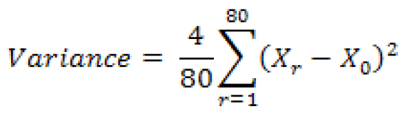
X0 is the estimate calculated using the production weight and Xr is the estimate calculated using the rth replicate weight. The standard error is the square root of the variance. The 90th percent margin of error is 1.645 times the standard error.
For more information on the formation of the replicate weights, see chapter 12 of the Design and Methodology documentation at http://www.census.gov/acs/www/Downloads/survey_methodology/Chapter_12_RevisedDec2010.pdf.
Beginning with the ACS 2011 1-year estimates, a new imputation-based methodology was incorporated into processing (see the description in the Group Quarters Person Weighting Section). An adjustment was made to the production replicate weight variance methodology to account for the non-negligible amount of additional variation being introduced by the new technique.5
Excluding the base weights, replicate weights were allowed to be negative in order to avoid underestimating the standard error. Exceptions include:
1. The estimate of the number or proportion of people, households, families, or housing units in a geographic area with a specific characteristic is zero. A special procedure is used to estimate the standard error.
2. There are either no sample observations available to compute an estimate or standard error of a median, an aggregate, a proportion, or some other ratio, or there are too few sample observations to compute a stable estimate of the standard error. The estimate is represented in the tables by "-" and the margin of error by "**" (two asterisks).
3. The estimate of a median falls in the lower open-ended interval or upper open-ended interval of a distribution. If the median occurs in the lowest interval, then a "-" follows the estimate, and if the median occurs in the upper interval, then a "+" follows the estimate. In both cases the margin of error is represented in the tables by "***" (three asterisks).
5For more information regarding this issue, see Asiala, M. and Castro, E. 2012. Developing Replicate Weight- Based Methods to Account for Imputation Variance in a Mass Imputation Application. In JSM proceedings, Section on Survey Research Methods, Alexandria, VA: American Statistical Association.
The standard error of the sum of two sample estimates is the square root of the sum of the two individual standard errors squared plus a covariance term. That is, for standard errors
 and
and of estimates
 and
and 

The covariance measures the interactions between two estimates. Currently the covariance terms are not available. Data users should use the approximation:
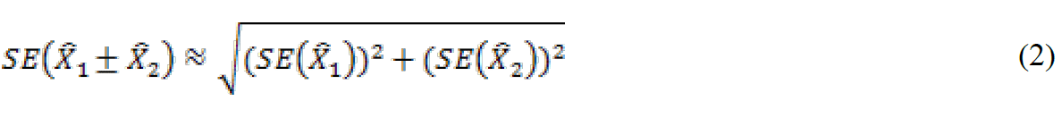
However, this method will underestimate or overestimate the standard error if the two estimates interact in either a positive or negative way.
The approximation formula (2) can be expanded to more than two estimates by adding in the individual standard errors squared inside the radical. As the number of estimates involved in the sum or difference increases, the results of formula (2) become increasingly different from the standard error derived directly from the ACS microdata. Care should be taken to work with the fewest number of estimates as possible. If there are estimates involved in the sum that are controlled in the weighting then the approximate standard error can be increasingly different. Several examples are provided starting on page 32 to demonstrate issues associated with approximating the standard errors when summing large numbers of estimates together.
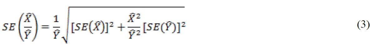
 , then the standard error of this proportion is approximated as:
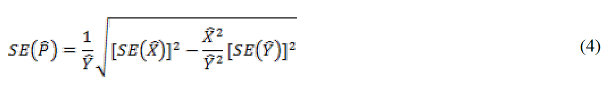
If
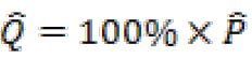 (P is the proportion and Q is its corresponding percent), then
 . Note the difference between the formulas to approximate the standard error for proportions (4) and ratios (3) - the plus sign in the previous formula has been replaced with a minus sign. If the value under the radical is negative, use the ratio standard error formula above, instead.
Let the current estimate
 and the earlier estimate
  then the formula for percent change is:
This reduces to a ratio. The ratio formula above may be used to calculate the standard error. As a caveat, this formula does not take into account the correlation when calculating overlapping time periods.
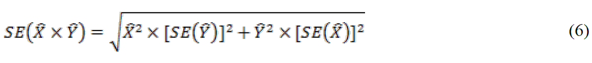
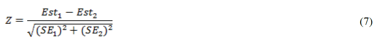
If Z > 1.645 or Z < -1.645, then the difference can be said to be statistically significant at the 90 percent confidence level. 6
Users are also cautioned to not rely on looking at whether confidence intervals for two estimates overlap or not to determine statistical significance, because there are circumstances where that method will not give the correct test result. If two confidence intervals do not overlap, then the estimates will be significantly different (i.e. the significance test will always agree). However, if two confidence intervals do overlap, then the estimates may or may not be significantly different.
The Z calculation above is recommended in all cases.
Here is a simple example of why it is not recommended to use the overlapping confidence bounds rule of thumb as a substitute for a statistical test.
Let: X1 = 6.0 with SE1 = 0.5 and X2 = 5.0 with SE2 = 0.2.
The Lower Bound for X12 = 5.0 + 0.2 x 1.645 = 5.3. The confidence bounds overlap, so, the rule of thumb would indicate that the estimates are not significantly different at the 90% level.
However, if we apply the statistical significance test we obtain:
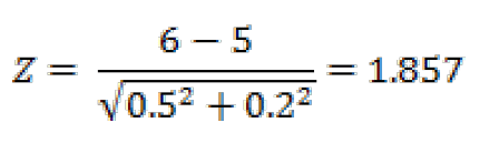
Z = 1.857 > 1.645 which means that the difference is significant (at the 90% level).
All statistical testing in ACS data products is based on the 90 percent confidence level. Users should understand that all testing was done using unrounded estimates and standard errors, and it may not be possible to replicate test results using the rounded estimates and margins of error as published.
6The ACS Accuracy of the Data document in 2005 used a Z statistic of +/-1.65. Data users should use +/-1.65 for estimates published in 2005 or earlier.
Standard Error = Margin of Error / 1.645
Calculating the standard error using the margin of error, we have:
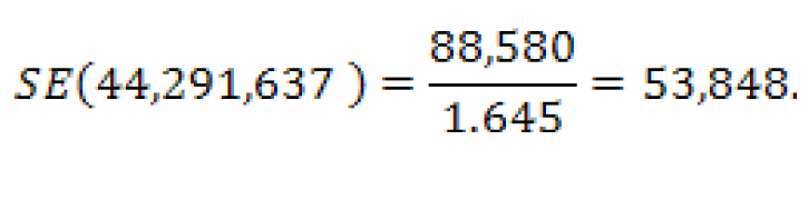

So using formula (2) for the approximate standard error of a sum or difference we have:
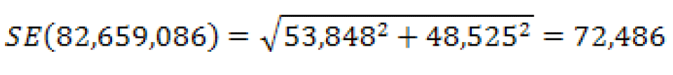
Caution: This method will underestimate or overestimate the standard error if the two estimates interact in either a positive or negative way.
To calculate the lower and upper bounds of the 90 percent confidence interval around 82,659,086 using the standard error, simply multiply 72,486 by 1.645, then add and subtract the product from 82,659,086. Thus the 90 percent confidence interval for this estimate is [82,659,086- 1.645(72,486)] to [82,659,086+ 1.645(72,486)] or 82,539,847 to 82,778,325.
The estimate is

So, using formula (4) for the approximate standard error of a proportion or percent, we have:

To calculate the lower and upper bounds of the 90 percent confidence interval around 46.42 using the standard error, simply multiply 0.04 by 1.645, then add and subtract the product from 46.42. Thus the 90 percent confidence interval for this estimate is [46.42 - 1.645(0.04)] to [46.42 + 1.645(0.04)], or 46.35 to 46.49.
The estimate of the ratio is 44,291,637 / 38,367,449 = 1.154.
Using formula (3) for the approximate standard error of this ratio we have:
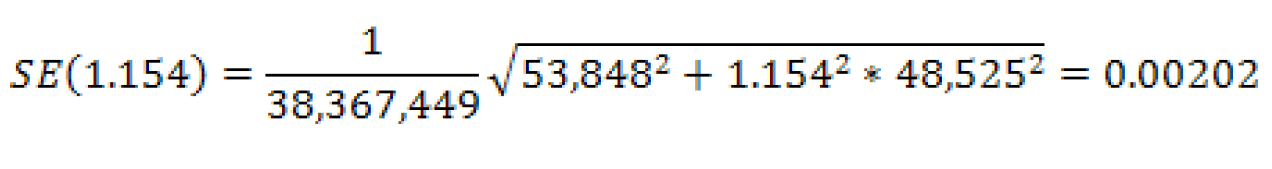
The 90 percent margin of error for this estimate would be 0.00202 multiplied by 1.645, or about 0.003. The 90 percent lower and upper 90 percent confidence bounds would then be [1.154 - 1.645(0.00202)] to [1.154 + 1.645(0.00202)], or 1.151 and 1.157.

and

The approximate standard error for number of 1-unit detached owner-occupied housing units is calculated using formula (5) for products as:

To calculate the lower and upper bounds of the 90 percent confidence interval around 61,000,148 using the standard error, simply multiply 111,848 by 1.645, then add and subtract the product from 61,000,148. Thus the 90 percent confidence interval for this estimate is [61,000,148 - 1.645(111,848)] to [61,000,148 + 1.645(111,848)] or 60,816,158 to 61,184,138.
- Coverage Error
A major way to avoid coverage error in a survey is to ensure that its sampling frame, for ACS an address list in each state, is as complete and accurate as possible. The source of addresses for the ACS is the MAF. An attempt is made to assign all appropriate geographic codes to each MAF address via an automated procedure using the Census Bureau TIGER (Topologically Integrated Geographic Encoding and Referencing) files. A manual coding operation based in the appropriate regional offices is attempted for addresses which could not be automatically coded. The MAF was used as the source of addresses for selecting sample housing units and mailing questionnaires. TIGER produced the location maps for CAPI assignments. Sometimes the MAF has an address that is the duplicate of another address already on the MAF. This could occur when there is a slight difference in the address such as 123 Main Street versus 123 Maine Street.
In the CATI and CAPI nonresponse follow-up phases, efforts were made to minimize the chances that housing units that were not part of the sample were interviewed in place of units in sample by mistake. If a CATI interviewer called a mail nonresponse case and was not able to reach the exact address, no interview was conducted and the case was eligible for CAPI. During CAPI follow-up, the interviewer had to locate the exact address for each sample housing unit. If the interviewer could not locate the exact sample unit in a multi-unit structure, or found a different number of units than expected, the interviewers were instructed to list the units in the building and follow a specific procedure to select a replacement sample unit. Person overcoverage can occur when an individual is included as a member of a housing unit but does not meet ACS residency rules.
Coverage rates give a measure of undercoverage or overcoverage of persons or housing units in a given geographic area. Rates below 100 percent indicate undercoverage, while rates above 100 percent indicate overcoverage. Coverage rates are released concurrent with the release of estimates on American FactFinder in the B98 series of detailed tables. Further information about ACS coverage rates may be found at http://www.census.gov/acs/www/methodology/methodology_main/.
- Nonresponse Error
- Unit Nonresponse - Unit nonresponse is the failure to obtain data from housing units in the sample. Unit nonresponse may occur because households are unwilling or unable to participate, or because an interviewer is unable to make contact with a housing unit. Unit nonresponse is problematic when there are systematic or variable differences between interviewed and noninterviewed housing units on the characteristics measured by the survey. Nonresponse bias is introduced into an estimate when differences are systematic, while nonresponse error for an estimate evolves from variable differences between interviewed and noninterviewed households.
The ACS makes every effort to minimize unit nonresponse, and thus, the potential for nonresponse error. First, the ACS used a combination of mail, CATI, and CAPI data collection modes to maximize response. The mail phase included a series of three to four mailings to encourage housing units to return the questionnaire. Subsequently, mail nonrespondents (for which phone numbers are available) were contacted by CATI for an interview. Finally, a subsample of the mail and telephone nonrespondents was contacted by personal visit to attempt an interview. Combined, these three efforts resulted in a very high overall response rate for the ACS.
ACS response rates measure the percent of units with a completed interview. The higher the response rate, and consequently the lower the nonresponse rate, the less chance estimates may be affected by nonresponse bias. Response and nonresponse rates, as well as rates for specific types of nonresponse, are released concurrent with the release of estimates on American FactFinder in the B98 series of detailed tables. Further information about response and nonresponse rates may be found at http://www.census.gov/acs/www/methodology/methodology_main/.
- Item Nonresponse - Nonresponse to particular questions on the survey questionnaire and instrument allows for the introduction of error or bias into the data, since the characteristics of the nonrespondents have not been observed and may differ from those reported by respondents. As a result, any imputation procedure using respondent data may not completely reflect this difference either at the elemental level (individual person or housing unit) or on average.
Some protection against the introduction of large errors or biases is afforded by minimizing nonresponse. In the ACS, item nonresponse for the CATI and CAPI operations was minimized by the requirement that the automated instrument receive a response to each question before the next one could be asked. Questionnaires returned by mail were edited for completeness and acceptability. They were reviewed by computer for content omissions and population coverage. If necessary, a telephone follow-up was made to obtain missing information. Potential coverage errors were included in this follow-up.
Allocation tables provide the weighted estimate of persons or housing units for which a value was imputed, as well as the total estimate of persons or housing units that were eligible to answer the question. The smaller the number of imputed responses, the lower the chance that the item nonresponse is contributing a bias to the estimates. Allocation tables are released concurrent with the release of estimates on American Factfinder in the B99 series of detailed tables with the overall allocation rates across all person and housing unit characteristics in the B98 series of detailed tables. Additional information on item nonresponse and allocations can be found at http://www.census.gov/acs/www/methodology/methodology_main/.
- Measurement and Processing Error
- Interviewer monitoring - The interviewer may misinterpret or otherwise incorrectly enter information given by a respondent; may fail to collect some of the information for a person or household; or may collect data for households that were not designated as part of the sample. To control these problems, the work of interviewers was monitored carefully. Field staff were prepared for their tasks by using specially developed training packages that included hands-on experience in using survey materials. A sample of the households interviewed by CAPI interviewers was reinterviewed to control for the possibility that interviewers may have fabricated data.
- Processing Error - The many phases involved in processing the survey data represent potential sources for the introduction of nonsampling error. The processing of the survey questionnaires includes the keying of data from completed questionnaires, automated clerical review, follow-up by telephone, manual coding of write-in responses, and automated data processing. The various field, coding and computer operations undergo a number of quality control checks to insure their accurate application.
- Content Editing - After data collection was completed, any remaining incomplete or inconsistent information was imputed during the final content edit of the collected data. Imputations, or computer assignments of acceptable codes in place of unacceptable entries or blanks, were needed most often when an entry for a given item was missing or when the information reported for a person or housing unit on that item was inconsistent with other information for that same person or housing unit. As in other surveys and previous censuses, the general procedure for changing unacceptable entries was to allocate an entry for a person or housing unit that was consistent with entries for persons or housing units with similar characteristics. Imputing acceptable values in place of blanks or unacceptable entries enhances the usefulness of the data.
A. Suppose we wish to estimate the total number of males with income below the poverty level in the past 12 months using both state and PUMA level estimates for the state of Wyoming. Part of the collapsed table C17001 is displayed below with estimates and their margins of error in parentheses.
Table A: 2009 Estimates of Males with Income Below Poverty from table C17001: Poverty Status in the Past 12 Months by Sex by Age
| Characteristic | Wyoming | PUMA 00100 | PUMA 00200 | PUMA 00300 | PUMA 00400 |
| Male | 23,001 (3,309) | 5,264 (1,624) | 6,508 (1,395) | 4,364 (1,026) | 6,865 (1,909) |
| Under 18 Years Old | 8,479 (1,874) | 2,041 (920) | 2,222 (778) | 1,999 (750) | 2,217 (1,192) |
| 18 to 64 Years Old | 12,976 (2,076) | 3,004 (1,049) | 3,725 (935) | 2,050 (635) | 4,197 (1,134) |
| 65 Years and Older | 1546 (500) | 219 (237) | 561 (286) | 315 (173) | 451 (302) |
| 2009 American FactFinder | |||||
The first way is to sum the three age groups for Wyoming:
Estimate(Male) = 8,479 + 12,976 + 1,546 = 23,001.
The first approximation for the standard error in this case gives us:
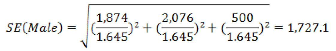
A second way is to sum the four PUMA estimates for Male to obtain:
Estimate(Male) = 5,264 + 6,508 + 4,364 + 6,865 = 23,001 as before.
The second approximation for the standard error yields:
Finally, we can sum up all three age groups for all four PUMAs to obtain an estimate based on a total of twelve estimates:

And the third approximated standard error is
However, we do know that the standard error using the published MOE is 3,309 /1.645 = 2,011.6. In this instance, all of the approximations under-estimate the published standard error and should be used with caution.
B. Suppose we wish to estimate the total number of males at the national level using age and citizenship status. The relevant data from table B05003 is displayed in table B below.
Table B: 2009 Estimates of males from B05003: Sex by Age by Citizenship Status
| Characteristic | Estimate | MOE |
| Male | 151,375,321 | 27,279 |
| Under 18 Years | 38,146,514 | 24,365 |
| Native | 36,747,407 | 31,397 |
| Foreign Born | 1,399,107 | 20,177 |
| Naturalized U.S. Citizen | 268,445 | 10,289 |
| Not a U.S. Citizen | 1,130,662 | 20,228 |
| 18 Years and Older | 113,228,807 | 23,525 |
| Native | 95,384,433 | 70,210 |
| Foreign Born | 17,844,374 | 59,750 |
| Naturalized U.S. Citizen | 7,507,308 | 39,658 |
| Not a U.S. Citizen | 10,337,066 | 65,533 |
| 2009 American FactFinder | ||
The estimate and its MOE are actually published. However, if they were not available in the tables, one way of obtaining them would be to add together the number of males under 18 and over 18 to get:

And the first approximated standard error is
Another way would be to add up the estimates for the three subcategories (Native, and the two subcategories for Foreign Born: Naturalized U.S. Citizen, and Not a U.S. Citizen), for males under and over 18 years of age. From these six estimates we obtain:
With a second approximated standard error of:
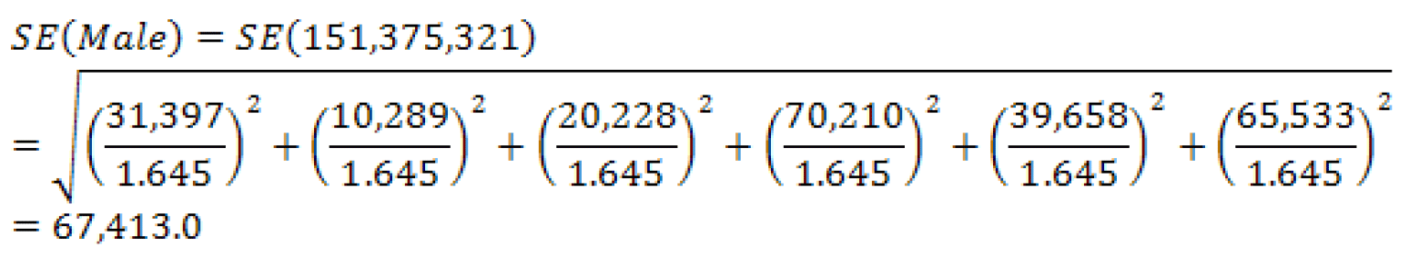
We do know that the standard error using the published margin of error is 27,279 / 1.645 = 16,583.0. With a quick glance, we can see that the ratio of the standard error of the first method to the published-based standard error yields 1.24; an over-estimate of roughly 24%, whereas the second method yields a ratio of 4.07 or an over-estimate of 307%. This is an example of what could happen to the approximate SE when the sum involves a controlled estimate. In this case, it is sex by age.
C. Suppose we are interested in the total number of people aged 65 or older and its standard error. Table C shows some of the estimates for the national level from table B01001 (the estimates in gray were derived for the purpose of this example only).
Table C: Some Estimates from AFF Table B01001: Sex by Age for 2009
| Age Category | Estimate, Male | MOE, Male | Estimate, Female | MOE, Female | Total | Estimated MOE, Total |
| 65 and 66 years old | 2,492,871 | 20,194 | 2,803,516 | 23,327 | 5,296,387 | 30,854 |
| 67 to 69 years old | 3,029,709 | 18,280 | 3,483,447 | 24,287 | 6,513,225 | 30,398 |
| 70 to 74 years old | 4,088,428 | 21,588 | 4,927,666 | 26,867 | 9,016,094 | 34,466 |
| 75 to 79 years old | 3,168,175 | 19,097 | 4,204,401 | 23,024 | 7,372,576 | 29,913 |
| 80 to 84 years old | 2,258,021 | 17,716 | 3,538,869 | 25,423 | 5,796,890 | 30,987 |
| 85 years and older | 1,743,971 | 17,991 | 3,767,574 | 19,294 | 5,511,545 | 26,381 |
| Total | 16,781,175 | NA | 22,725,473 | NA | 39,506,648 | 74,932 |
| 2009 American FactFinder | ||||||
To begin we find the total number of people aged 65 and over by simply adding the totals for males and females to get 16,781,175 + 22,725,542 = 39,506,717. One way we could use is summing males and female for each age category and then using their MOEs to approximate the standard error for the total number of people over 65.
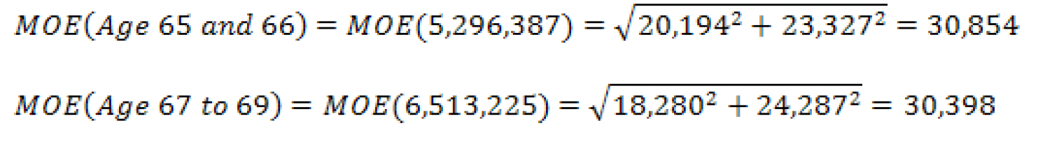
... etc. ...
Now, we calculate for the number of people aged 65 or older to be 39,506,648 using the six derived estimates and approximate the standard error:
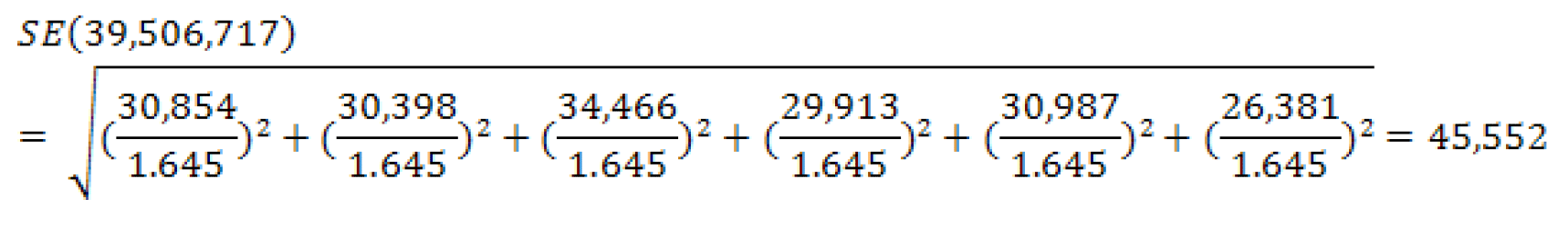
For this example the estimate and its MOE are published in table B09017. The total number of people aged 65 or older is 39,506,648 with a margin of error of 20,689. Therefore the published- based standard error is:
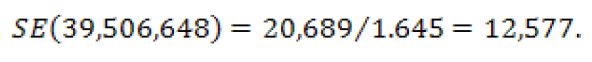
The approximated standard error, using six derived age group estimates, yields an approximated standard error roughly 3.6 times larger than the published-based standard error.
As a note, there are two additional ways to approximate the standard error of people aged 65 and over in addition to the way used above. The first is to find the published MOEs for the males age 65 and older and of females aged 65 and older separately and then combine to find the approximate standard error for the total. The second is to use all twelve of the published estimates together, that is, all estimates from the male age categories and female age categories, to create the SE for people aged 65 and older. However, in this particular example, the results from all three ways are the same. So no matter which way you use, you will obtain the same approximation for the SE. This is different from the results seen in example A.
D. For an alternative to approximating the standard error for people 65 years and older seen in part C, we could find the estimate and its SE by summing all of the estimate for the ages less than 65 years old and subtracting them from the estimate for the total population. Due to the large number of estimates, Table D does not show all of the age groups. In addition, the estimates in part of the table shaded gray were derived for the purposes of this example only and cannot be found in base table B01001.
Table D: Some Estimates from AFF Table B01001: Sex by Age for 2009:
| Age Category | Estimate, Male | MOE, Male | Estimate, Female | MOE, Female | Total | Estimated MOE, Total |
| Total Population | 151,375,321 | 27,279 | 155,631,235 | 27,280 | 307,006,556 | 38,579 |
| Under 5 years | 10,853,263 | 15,661 | 10,355,944 | 14,707 | 21,209,207 | 21,484 |
| 5 to 9 years old | 10,273,948 | 43,555 | 9,850,065 | 42,194 | 20,124,013 | 60,641 |
| 10 to 14 years old | 10,532,166 | 40,051 | 9,985,327 | 39,921 | 20,517,493 | 56,549 |
| ... | ... | ... | ... | ... | ||
| 62 to 64 years old | 4,282,178 | 25,636 | 4,669,376 | 28,769 | 8,951,554 | 38,534 |
| Total for Age 0 to 64 years old | 134,594,146 | 117,166 | 132,905,762 | 117,637 | 267,499,908 | 166,031 |
| Total for Age 65 years and older | 16,781,175 | 120,300 | 22,725,473 | 120,758 | 39,506,648 | 170,454 |
| 2009 American FactFinder | ||||||
An estimate for the number of people age 65 and older is equal to the total population minus the population between the ages of zero and 64 years old:
Number of people aged 65 and older: 307,006,556 - 267,499,908 = 39,506,648.
The way to approximate the SE is the same as in part C. First we will sum male and female estimates across each age category and then approximate the MOEs. We will use that information to approximate the standard error for our estimate of interest:
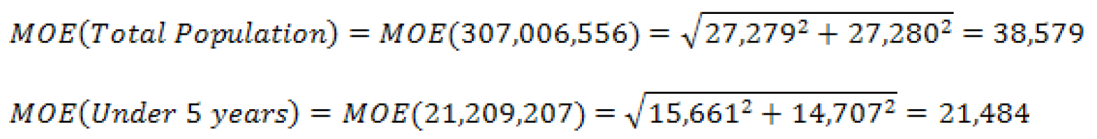
... etc. ...
And the SE for the total number of people aged 65 and older is:
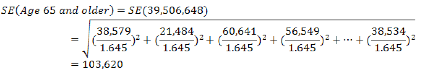
Again, as in Example C, the estimate and its MOE are we published in B09017. The total number of people aged 65 or older is 39,506,648 with a margin of error of 20,689. Therefore the standard error is:

The approximated standard error using the thirteen derived age group estimates yields a standard error roughly 8.2 times larger than the actual SE.
Data users can mitigate the problems shown in examples A through D to some extent by utilizing a collapsed version of a detailed table (if it is available) which will reduce the number of estimates used in the approximation. These issues may also be avoided by creating estimates and SEs using the Public Use Microdata Sample (PUMS) or by requesting a custom tabulation, a fee- based service offered under certain conditions by the Census Bureau. More information regarding custom tabulations may be found at http://www.census.gov/acs/www/data_documentation/custom_tabulations/.
Additional information on the design and methodology of the PRCS, including data collection and processing, can be found at:
http://www.census.gov/acs/www/methodology/methodology_main/.
The 2012 Accuracy of the Data for the United States can be found at:
http://www.census.gov/acs/www/Downloads/data_documentation/Accuracy/PRCS_Accuracy_of_Data_2012.pdf.
- Mailout/Mailback
- Computer Assisted Telephone Interview (CATI)
- Computer Assisted Personal Interview (CAPI)
Month 1: Addresses in sample that are determined to be mailable are sent a questionnaire via
the U.S. Postal Service.
Month 2: All mail non-responding addresses with an available phone number are sent to CATI.
Month 3: A sample of mail non-responses without a phone number, CATI non-responses, and unmailable addresses are selected and sent to CAPI.
Note that mail responses are accepted during all three months of data collection.
Group Quarters data collection spans six weeks, except for Federal prisons, where the data collection time period is four months. All Federal prisons are assigned to September with a four month data collection window.
- Soup kitchens
- Domestic violence shelters
- Regularly scheduled mobile food vans
- Targeted non-sheltered outdoor locations
- Maritime/merchant vessels
- Living quarters for victims of natural disasters
Several of the steps used to select the first-phase sample are common to both Main and Supplemental sampling. The descriptions of the steps included in the first-phase sample selection below indicate which are common to both and which are unique to either Main or Supplemental sampling.
1. First-phase Sample Selection
- First-stage sampling (performed during both Main and Supplemental sampling) - First stage sampling defines the universe for the second stage of sampling through two steps. First, all addresses that were in a first-phase sample within the past four years are excluded from eligibility. This ensures that no address is in sample more than once in any five-year period. The second step is to select a 20 percent systematic sample of "new" units, i.e. those units that have never appeared on a previous MAF extract. Each new address is systematically assigned to either the current year or to one of four back- samples. This procedure maintains five equal partitions of the universe.
- Assignment of blocks to a second-stage sampling stratum (performed during Main sampling only) - Second-stage sampling uses five sampling strata in PR. The stratum level rates used in second-stage sampling account for the first-stage selection probabilities. These rates are applied at a block level to addresses in PR by calculating a measure of size for Municipios.
The measure of size is an estimate of the number of occupied HUs in the Municipio. This is calculated by multiplying the number of PRCS addresses by the occupancy rate from the 2010 Census at the block level. A measure of size for each Census Tract is also calculated in the same manner.
Each block is then assigned the smallest measure of size from the set of all entities of which it is a part. The second-stage sampling strata and the overall first-phase sampling rates are shown in Table 1 below.
- Calculation of the second-stage sampling rates (performed during Main sampling only) - The overall first-phase sampling rates given in Table 1 are calculated using the distribution of PRCS valid addresses by second-stage sampling stratum in such a way as to yield an overall target sample size for the year of approximately 36,000. The first- phase rates are adjusted for the first-stage sample to yield the second-stage selection probabilities.
- Second-stage sample selection (performed in Main and Supplemental) - After each block is assigned to a second-stage sampling stratum, a systematic sample of addresses is selected from the second-stage universe (first-stage sample) within each municipio.
- Sample Month Assignment (performed in Main and Supplemental) - After the second stage of sampling, all sample addresses are randomly assigned to a sample month. Addresses selected during Main sampling are allocated to each of the 12 months.
| Sampling Stratum | Type of Area | Rate Definitions | 2012 Sampling Rate |
| 1 | 0 < MOS1 ≤ 200 | 15% | 15.00% |
| 2 | 200 < MOS ≤ 400 | 10% | 10.00% |
| 3 | 400 < MOS ≤ 800 | 7% | 7.00% |
| 4 | 800 < MOS ≤ 1,200 | 2.8 × BR | 3.95% |
| 5 | 0 < TRACTMOS2 ≤ 400 | 3.5 × BR | 4.94% |
| 7 | 400 < TRACTMOS ≤ 1,000 | 2.8 × BR | 3.95% |
| 9 | 1,000 < TRACTMOS ≤ 2,000 | 1.7 × BR | 2.40% |
| 11 | 2,000 < TRACTMOS ≤ 4,000 | BR3 | 1.41% |
| 13 | 4,000 < TRACTMOS ≤ 6,000 | 0.6 × BR | 0.85% |
| 15 | 6,000 < TRACTMOS | 0.35 × BR | 0.49% |
| Note: A subset of sampling strata is listed here since not all of the stateside sampling strata are defined in Puerto Rico. | |||
| 1MOS = measure of size (estimated number occupied housing units) of the smallest governmental entity | |||
| 2TRACTMOS = the measure of size (MOS) at the Census Tract level | |||
| 3BR = base sampling rate | |||
2. Second-phase Sample Selection - Subsampling the Unmailable and Non-Responding Addresses
All addresses determined to be unmailable are subsampled for the CAPI phase of data collection at a rate of 2-in-3. Unmailable addresses do not go to the CATI phase of data collection. All addresses for which no response has been obtained prior to CAPI are subsampled at a rate of 1-in-2. Puerto Rico CAPI rates are summarized in Table 2.
Table 2. Second-Phase (CAPI) Subsampling Rates for Puerto Rico
| Address Characteristics | CAPI Subsampling Rate |
| Unmailable addresses | 66.7% |
| Mailable addresses | 50.0% |
1.First-phase Sample Selection for Small GQ Stratum
- First-stage sampling - Small GQs are only eligible to be selected for the PRCS once every five years. To accomplish this, the first stage sampling procedure systematically assigned all small GQs to one of five partitions of the universe. Each partition was assigned to a particular year (2012-2016) and the one assigned to 2012 became the first stage sample. In future years, each new GQ will be systematically assigned to one of the five samples. These samples are rotated over five year periods and become the universe for selecting the second stage sample.
- Second-stage sampling - A simple 1-in-8 systematic sample of the GQs in the first stage sample is selected. Regardless of their actual size, all GQs in the small stratum have the same probability of selection. Since the first stage sample is 20% of the universe, this yields the targeted sampling rate of 2.5%.
2.Sample Selection for the Large GQ Stratum
Unlike housing unit address sampling and the small GQ sample selection, the large GQ sampling procedure has no first-stage in which sampling units are randomly assigned to one of five years. All large GQs are eligible for sampling each year. The large GQ samples are selected using a two-phase design.
- First-phase Sampling
3.Sample Month Assignment
In order to assign a panel month to each hit, all of the GQ samples from Puerto Rico are combined and sorted by small/large stratum and second-phase order of selection.
Consecutive samples are assigned to the twelve panel months in a predetermined order, starting with a randomly determined month, except for Federal prisons. Correctional facilities have their sample clustered. All Federal prisons hits are assigned to the September panel. In non-Federal correctional facilities, all hits for a given GQ are assigned to the same panel month. However, unlike Federal prisons, the hits in state and local correctional facilities are assigned to randomly selected panels spread throughout the year.
4. Second Phase Sample: Selection of Persons in Small and Large GQs
Small GQs in the second phase sampling are "take all," i.e., every person in the selected GQ is eligible to receive a questionnaire. If the actual number of persons in the GQ exceeds 15, a field subsampling operation is performed to reduce the total number of sample persons interviewed at the GQ to 10. If the actual number of persons in the GQ is 15 or less, all people in the GQ will receive the questionnaire.
For each hit in the large GQs, the automated instrument uses the population count at the time of the visit and selects a subsample of 10 people from the roster. The people in this subsample receive the questionnaire.
The weighting is conducted in two main operations: a group quarters person weighting operation which assigns weights to persons in group quarters, and a household person weighting operation which assigns weights both to housing units and to persons within housing units. The group quarters person weighting is conducted first and the household person weighting second. The household person weighting is dependent on the group quarters person weighting because estimates for total population, which include both group quarters and household population, are controlled to the Census Bureau's official 2012 total resident population estimates.
supplemented by a large-scale whole person imputation into not-in-sample GQ facilities. For the 2012 PRCS GQ data, roughly as many GQ persons were imputed as sampled. The goal of the imputation methodology was two-fold.
1.The primary objective was to establish representation of municipio by major GQ type group in the tabulations for each combination that exists on the PRCS GQ sample frame. The seven major GQ type groups are defined by the Population Estimates Program and are given in Table 4.
2.A secondary objective was to establish representation of tract by major GQ type group for each combination that exists on the PRCS GQ sample frame.
Table 4: Population Estimates Program Major GQ Type Groups
| Major GQ Type Group | Definition | Institutional / Non-Institutional |
| 1 | Correctional Institutions | Institutional |
| 2 | Juvenile Detention Facilities | Institutional |
| 3 | Nursing Homes | Institutional |
| 4 | Other Long-Term Care Facilities | Institutional |
| 5 | College Dormitories | Non-Institutional |
| 6 | Military Facilities | Non-Institutional |
| 7 | Other Non-Institutional Facilities | Non-Institutional |
For all not-in-sample GQ facilities with an expected population of 16 or more persons (large facilities), we imputed a number of GQ persons equal to 2.5% of the expected population. For those GQ facilities with an expected population of fewer than 16 persons (small facilities), we selected a random sample of GQ facilities as needed to accomplish the two objectives given above. For those selected small GQ facilities, we imputed a number of GQ persons equal to 20% of the facilitys expected population.
Interviewed GQ person records were then sampled at random to be imputed into the selected not-in-sample GQ facilities. An expanding search algorithm searched for donors within the same specific type of GQ facility and the same municipio. If that failed, the search included all GQ facilities of the same major GQ type group. If that still failed, the search expanded to a specific type within a larger geography, then a major GQ type group within that geography, and so on until suitable donors were found.
The weighting procedure made no distinction between sampled and imputed GQ person records. The initial weights of person records in the large GQ facilities equaled the observed or expected population of the GQ facility divided by the number of person records. The initial weights of person records in small GQ facilities equaled the observed or expected population of the GQ facility divided by the number of records, multiplied by the inverse of the fraction represented on the frame of the small GQ facilities of that tract by major GQ type group combination. As was done in previous years weighting, we controlled the final weights to an independent set of GQ population estimates produced by the Population Estimates Program for each state by each of the seven major GQ type groups.
Lastly, the final GQ person weight was rounded to an integer. Rounding was performed so that the sum of the rounded weights were within one person of the sum of the unrounded weights for any of the groups listed below:
Major GQ Type Group
Major GQ Type Group x Municipio
- Percent in poverty (the only characteristic using ACS 5-year data)
- Percent renting
- Density of housing units (a proxy for rural areas)
- Race, ethnicity, age, and sex distribution
- Distance between the centroids of the counties
- Core-based Statistical Area status
The estimation procedure used to assign the weights is then performed independently within each of the PRCS weighting areas.
1. Initial Housing Unit Weighting Factors-This process produces the following factors:
- Base Weight (BW) - This initial weight is assigned to every housing unit as the inverse of its block's sampling rate.
- CAPI Subsampling Factor (SSF) - The weights of the CAPI cases are adjusted to reflect the results of CAPI subsampling. This factor is assigned to each record as follows:
Selected in CAPI subsampling: SSF = 2.0
Not selected in CAPI subsampling: SSF = 0.0
Not a CAPI case: SSF = 1.0
Some sample addresses are unmailable. A two-thirds sample of these is sent directly to CAPI and for these cases SSF = 1.5.
- Variation in Monthly Response by Mode (VMS)-This factor makes the total weight of the Mail, CATI, and CAPI records to be tabulated in a month equal to the total base weight of all cases originally mailed for that month. For all cases, VMS is computed and assigned based on the following groups:
Weighting Area x Month
- Noninterview Factor (NIF)-This factor adjusts the weight of all responding occupied housing units to account for nonresponding housing units. The factor is computed in two stages. The first factor, NIF1, is a ratio adjustment that is computed and assigned to occupied housings units based on the following groups:
A second factor, NIF2, is a ratio adjustment that is computed and assigned to occupied housing units based on the following groups:
Weighting Area x Building Type x Month
NIF is then computed by applying NIF1 and NIF2 for each occupied housing unit. Vacant housing units are assigned a value of NIF = 1.0. Nonresponding housing units are assigned a weight of 0.0.
- Noninterview Factor - Mode (NIFM) - This factor adjusts the weight of the responding CAPI occupied housing units to account for CAPI nonrespondents. It is computed as if NIF had not already been assigned to every occupied housing unit record. This factor is not used directly but rather as part of computing the next factor, the Mode Bias Factor.
Weighting Area x Building Type (single or multi unit) x MonthVacant housing units or non-CAPI (mail and CATI) housing units receive a value of NIFM = 1.0.
- Mode Bias Factor (MBF)-This factor makes the total weight of the housing units in the groups below the same as if NIFM had been used instead of NIF. MBF is computed and assigned to occupied housing units based on the following groups:
Vacant housing units receive a value of MBF = 1.0. MBF is applied to the weights computed through NIF.
- Housing unit Post-stratification Factor (HPF)-This factor makes the total weight of all housing units agree with the 2012 independent housing unit estimates at the subcounty level.
housing unit is the product of the weighting factors of their associated housing unit (BW x ... x MBF). At this point everyone in the household has the same weight. The person weighting is done in a series of three steps which are repeated until a stopping criterion is met. These three steps form a raking ratio or raking process. These person weights are individually adjusted for each person as described below.
The three steps are as follows:
- Municipio Controls Raking Factor (SUBEQRF) - This factor is applied to individuals based on their geography. It adjusts the person weights so that the weighted sample counts equal independent population estimates of total population for the municipio. For those municipios which are their own weighting area, this adjustment factor will be 1.0. Because of later adjustments to the person weights, total population is not assured of agreeing exactly with the official 2012 population estimates for municipios which are not their own weighting area.
- Spouse Equalization/Householder Equalization Raking Factor (SPHHEQRF)-This factor is applied to individuals based on the combination of their status of being in a married- couple or unmarried-partner household and whether they are the householder. All persons are assigned to one of four groups:
2.Spouse or unmarried partner in a married-couple or unmarried-partner household (non-householder)
3.Other householder
4.Other non-householder
The weights of persons in the first two groups are adjusted so that their sums are each equal to the total estimate of married-couple or unmarried-partner households using the housing unit weight (BW x ... x HPF). At the same time the weights of persons in the first and third groups are adjusted so that their sum is equal to the total estimate of occupied housing units using the housing unit weight (BW x ... x HPF). The goal of this step is to produce more consistent estimates of spouses or unmarried partners and married-couple and unmarried-partner households while simultaneously producing more consistent estimates of householders, occupied housing units, and households.
- Demographic Raking Factor (DEMORF)-This factor is applied to individuals based on their age and sex in Puerto Rico (note that there are 13 Age groupings). It adjusts the person weights so that the weighted sample counts equal the independent population estimates by age and sex at the weighting area level. Because of collapsing of groups in applying this factor, only the total population is assured of agreeing with the official 2012 population estimates at the weighting area level.
These three steps are repeated several times until the estimates for Puerto Rico achieve their optimal consistency with regard to the spouse and householder equalization. The Person Post-Stratification Factor (PPSF) is then equal to the product (SUBEQRF x SPHHEQRF x DEMORF) from all of iterations of these three adjustments. The unrounded person weight is then the equal to the product of PPSF times the housing unit weight (BW x ... x MBF x PPSF).
3.Rounding-The final product of all person weights (BW x ... x MBF x PPSF) is rounded to an integer. Rounding is performed so that the sum of the rounded weights is within one person of the sum of the unrounded weights for any of the groups listed below:
Municipio
Municipio x Sex
Municipio x Sex x Age
Municipio x Sex x Age x Tract
Municipio x Sex x Age x Tract x Block
For example, the number of Males, Age 30 estimated for a municipio using the rounded weights is within one of the number produced using the unrounded weights.
4.Final Housing Unit Weighting Factors-This process produces the following factors:
- Householder Factor (HHF)-This factor adjusts for differential response depending on the sex and age of the householder. The value of HHF for an occupied housing unit is the PPSF of the householder. Since there is no householder for vacant units, the value of HHF = 1.0 for all vacant units.
- Rounding-The final product of all housing unit weights (BW x ... x HHF) is rounded to an integer. For occupied units, the rounded housing unit weight is the same as the rounded person weight of the householder. This ensures that both the rounded and unrounded householder weights are equal to the occupied housing unit weight. The rounding for vacant housing units is then performed so that total rounded weight is within one housing unit of the total unrounded weight for any of the groups listed below:
Municipio
Municipio x Tract
Municipio x Tract x Block
The Census Bureau's internal Disclosure Review Board sets the confidentiality rules for all data releases. A checklist approach is used to ensure that all potential risks to the confidentiality of the data are considered and addressed.
- Title 13, United States Code: Title 13 of the United States Code authorizes the Census Bureau to conduct censuses and surveys. Section 9 of the same Title requires that any information collected from the public under the authority of Title 13 be maintained as confidential. Section 214 of Title 13 and Sections 3559 and 3571 of Title 18 of the United States Code provide for the imposition of penalties of up to five years in prison and up to $250,000 in fines for wrongful disclosure of confidential census information.
- Disclosure Avoidance: Disclosure avoidance is the process for protecting the confidentiality of data. A disclosure of data occurs when someone can use published statistical information to identify an individual that has provided information under a pledge of confidentiality. For data tabulations, the Census Bureau uses disclosure avoidance procedures to modify or remove the characteristics that put confidential information at risk for disclosure. Although it may appear that a table shows information about a specific individual, the Census Bureau has taken steps to disguise or suppress the original data while making sure the results are still useful. The techniques used by the Census Bureau to protect confidentiality in tabulations vary, depending on the type of data. All disclosure avoidance procedures are done prior to the whole person imputation into not-in-sample GQ facilities.
- Data Swapping: Data swapping is a method of disclosure avoidance designed to protect confidentiality in tables of frequency data (the number or percent of the population with certain characteristics). Data swapping is done by editing the source data or exchanging records for a sample of cases when creating a table. A sample of households is selected and matched on a set of selected key variables with households in neighboring geographic areas that have similar characteristics (such as the same number of adults and same number of children). Because the swap often occurs within a neighboring area, there is no effect on the marginal totals for the area or for totals that include data from multiple areas. Because of data swapping, users should not assume that tables with cells having a value of one or two reveal information about specific individuals. Data swapping procedures were first used in the 1990 Census, and were used again in Census 2000 and the 2010 Census.
- Synthetic Data: The goals of using synthetic data are the same as the goals of data swapping, namely to protect the confidentiality in tables of frequency data. Persons are identified as being at risk for disclosure based on certain characteristics. The synthetic data technique then models the values for another collection of characteristics to protect the confidentiality of that individual.
- Sampling Error - The data in the PRCS products are estimates of the actual figures that would have been obtained by interviewing the entire population using the same methodology. The estimates from the chosen sample also differ from other samples of housing units and persons within those housing units. Sampling error in data arises due to the use of probability sampling, which is necessary to ensure the integrity and representativeness of sample survey results. The implementation of statistical sampling procedures provides the basis for the statistical analysis of sample data. Measures used to estimate the sampling error are provided in the next section.
- Nonsampling Error - In addition to sampling error, data users should realize that other types of errors may be introduced during any of the various complex operations used to collect and process survey data. For example, operations such as data entry from questionnaires and editing may introduce error into the estimates. Another source is through the use of controls in the weighting. The controls are designed to mitigate the effects of systematic undercoverage of certain groups who are difficult to enumerate and to reduce the variance. The controls are based on the population estimates extrapolated from the previous census. Errors can be brought into the data if the extrapolation methods do not properly reflect the population. However, the potential risk from using the controls in the weighting process is offset by far greater benefits to the PRCS estimates. These benefits include reducing the effects of a larger coverage problem found in most surveys, including the PRCS, and the reduction of standard errors of PRCS estimates. These and other sources of error contribute to the nonsampling error component of the total error of survey estimates. Nonsampling errors may affect the data in two ways. Errors that are introduced randomly increase the variability of the data. Systematic errors which are consistent in one direction introduce bias into the results of a sample survey. The Census Bureau protects against the effect of systematic errors on survey estimates by conducting extensive research and evaluation programs on sampling techniques, questionnaire design, and data collection and processing procedures. In addition, an important goal of the PRCS is to minimize the amount of nonsampling error introduced through nonresponse for sample housing units. One way of accomplishing this is by following up on mail nonrespondents during the CATI and CAPI phases. For more information, see the section entitled "Control of Nonsampling Error".
Estimates of the magnitude of sampling errors - in the form of margins of error - are provided with all published PRCS data. The Census Bureau recommends that data users incorporate this information into their analyses, as sampling error in survey estimates could impact the conclusions drawn from the results.
For example, if all possible samples that could result under the PRCS sample design were independently selected and surveyed under the same conditions, and if the estimate and its estimated standard error were calculated for each of these samples, then:
1. Approximately 68 percent of the intervals from one estimated standard error below the estimate to one estimated standard error above the estimate would contain the average result from all possible samples;
2. Approximately 90 percent of the intervals from 1.645 times the estimated standard error below the estimate to 1.645 times the estimated standard error above the estimate would contain the average result from all possible samples.
3. Approximately 95 percent of the intervals from two estimated standard errors below the estimate to two estimated standard errors above the estimate would contain the average result from all possible samples.
The intervals are referred to as 68 percent, 90 percent, and 95 percent confidence intervals, respectively.
Margin of Error - Instead of providing the upper and lower confidence bounds in published PRCS tables, the margin of error is provided instead. The margin of error is the difference between an estimate and its upper or lower confidence bound. Both the confidence bounds and the standard error can easily be computed from the margin of error. All PRCS published margins of error are based on a 90 percent confidence level.
Standard Error = Margin of Error / 1.645
Lower Confidence Bound = Estimate - Margin of Error
Upper Confidence Bound = Estimate + Margin of Error
Note that for 2005, PRCS margins of error and confidence bounds were calculated using a 90 percent confidence level multiplier of 1.65. With the 2006 data release, and for every year after 2006, we now employ a more accurate multiplier of 1.645. Margins of error and confidence bounds from previously published products will not be updated with the new multiplier. When calculating standard errors from margins of error or confidence bounds using published data for 2005, use the 1.65 multiplier.
When constructing confidence bounds from the margin of error, the user should be aware of any "natural" limits on the bounds. For example, if a characteristic estimate for the population is near zero, the calculated value of the lower confidence bound may be negative. However, a negative number of people does not make sense, so the lower confidence bound should be reported as zero instead. However, for other estimates such as income, negative values do make sense. The context and meaning of the estimate must be kept in mind when creating these bounds. Another of these natural limits would be 100 percent for the upper bound of a percent estimate.
If the margin of error is displayed as '*****' (five asterisks), the estimate has been controlled to be equal to a fixed value and so it has no sampling error. When using any of the formulas in the following section, use a standard error of zero for these controlled estimates.
Limitations -The user should be careful when computing and interpreting confidence intervals.
- The estimated standard errors (and thus margins of error) included in these data products do not include portions of the variability due to nonsampling error that may be present in the data. In particular, the standard errors do not reflect the effect of correlated errors introduced by interviewers, coders, or other field or processing personnel. Nor do they reflect the error from imputed values due to missing responses. Thus, the standard errors calculated represent a lower bound of the total error. As a result, confidence intervals formed using these estimated standard errors may not meet the stated levels of confidence (i.e., 68, 90, or 95 percent). Thus, some care must be exercised in the interpretation of the data in this data product based on the estimated standard errors.
- Zero or small estimates; very large estimates - The value of almost all PRCS characteristics is greater than or equal to zero by definition. For zero or small estimates, use of the method given previously for calculating confidence intervals relies on large sample theory, and may result in negative values which for most characteristics are not admissible. In this case the lower limit of the confidence interval is set to zero by default. A similar caution holds for estimates of totals close to a control total or estimated proportion near one, where the upper limit of the confidence interval is set to its largest admissible value. In these situations the level of confidence of the adjusted range of values is less than the prescribed confidence level.
The formula provided below calculates the variance using the PRCS estimate (X0) and the 80 replicate estimates (Xr).
X0 is the estimate calculated using the production weight and Xr is the estimate calculated using the rth replicate weight. The standard error is the square root of the variance. The 90th percent margin of error is 1.645 times the standard error.
For more information on the formation of the replicate weights, see chapter 12 of the Design and Methodology documentation at http://www.census.gov/acs/www/Downloads/survey_methodology/Chapter_12_RevisedDec2010.pdf.
Beginning with the PRCS 2011 1-year estimates, a new imputation-based methodology was incorporated into processing (see the description in the Group Quarters Person Weighting Section). An adjustment was made to the production replicate weight variance methodology to account for the non-negligible amount of additional variation being introduced by the new technique. 1
Excluding the base weights, replicate weights were allowed to be negative in order to avoid underestimating the standard error. Exceptions include:
1. The estimate of the number or proportion of people, households, families, or housing units in a geographic area with a specific characteristic is zero. A special procedure is used to estimate the standard error.
2. There are either no sample observations available to compute an estimate or standard error of a median, an aggregate, a proportion, or some other ratio, or there are too few sample observations to compute a stable estimate of the standard error. The estimate is represented in the tables by "-" and the margin of error by "**" (two asterisks).
3. The estimate of a median falls in the lower open-ended interval or upper open-ended interval of a distribution. If the median occurs in the lowest interval, then a "-" follows the estimate, and if the median occurs in the upper interval, then a "+" follows the estimate. In both cases the margin of error is represented in the tables by "***" (three asterisks).
1 For more information regarding this issue, see Asiala, M. and Castro, E. 2012. Developing Replicate Weight- Based Methods to Account for Imputation Variance in a Mass Imputation Application. In JSM proceedings, Section on Survey Research Methods, Alexandria, VA: American Statistical Association.
The standard error of the sum of two sample estimates is the square root of the sum of the two individual standard errors squared plus a covariance term. That is, for standard errors
and of estimates and The covariance measures the interaction between two estimates. Currently the covariance terms are not available. Data users should use the approximation:
This method, however, will underestimate or overestimate the standard error if the two estimates interact in either a positive or negative way.
The approximation formula (2) can be expanded to more than two estimates by adding in the individual standard errors squared inside the radical. As the number of estimates involved in the sum or difference increases, the results of formula (2) become increasingly different from the standard error derived directly from the PRCS microdata. Care should be taken to work with the fewest number of estimates as possible. If there are estimates involved in the sum that are controlled in the weighting then the approximate standard error can be increasingly different. Several examples are provided starting on page 29 to demonstrate how issues associated with approximating the standard errors when summing large numbers of estimates together.
,then the standard error of this proportion is approximated as:If
(P is the proportion and Q is its corresponding percent), then . Note the difference between the formulas to approximate the standard error for proportions and ratios - the plus sign in the ratio formula has been replaced with a minus sign in proportions formula. If the value under the square root sign is negative, use the ratio standard error formula instead.
Let the current estimate
and the earlier estimate then the formula for percent change is:This reduces to a ratio. The ratio formula above may be used to calculate the standard error. As a caveat, this formula does not take into account the correlation when calculating overlapping time periods.
If Z > 1.645 or Z < -1.645, then the difference can be said to be statistically significant at the 90 percent confidence level. Any estimate can be compared to a PRCS estimate using this method, including other PRCS estimates from the current year, the PRCS estimate for the same characteristic and geographic area but from a previous year, ACS estimates, 2010 Census counts, estimates from other Census Bureau surveys, and estimates from other sources. Not all estimates have sampling error - 2010 Census counts do not - but they should be used if they exist to give the most accurate result of the test.
Users are also cautioned to not rely on looking at whether confidence intervals for two estimates overlap or not to determine statistical significance, because there are circumstances where that method will not give the correct test result. If two confidence intervals do not overlap, then the estimates will be significantly different (i.e. the significance test will always agree). However, if two confidence intervals do overlap, then the estimates may or may not be significantly different. The Z calculation above is recommended in all cases.
Here is a simple example of why it is not recommended to use the overlapping confidence bounds rule of thumb as a substitute for a statistical test.
Let: X1 = 6.0 with SE1 = 0.5 and X2 = 5.0 with SE2 = 0.2.
The Lower Bound for X12 = 5.0 + 0.2 x 1.645 = 5.3. The confidence bounds overlap, so, the rule of thumb would indicate that the estimates are not significantly different at the 90% level.
However, if we apply the statistical significance test we obtain:
Z = 1.857 > 1.645 which means that the difference is significant (at the 90% level).
All statistical testing in PRCS data products is based on the 90 percent confidence level. Users should understand that all testing was done using unrounded estimates and standard errors, and it may not be possible to replicate test results using the rounded estimates and margins of error as published.
Standard Error = Margin of Error / 1.645
Calculating the standard error using the margin of error, we have:
SE(587,937) = 7,168/ 1.645 = 4,357.
SE(550,748) = 9,095 / 1.645 = 5,529.
So using formula (2) for the approximate standard error of a sum or difference we have:
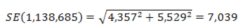
Caution: This method will underestimate or overestimate the standard error if the two estimates interact in either a positive or negative way.
To calculate the lower and upper bounds of the 90 percent confidence interval around 1,138,685 using the standard error, simply multiply 7,039 by 1.645, then add and subtract the product from 1,138,685. Thus the 90 percent confidence interval for this estimate is [1,138,685 - 1.645(7,039)] to [1,138,685 + 1.645(7,039)] or 1,127,106 to 1,150,264.
The estimate is (550,748 / 1,138,685) * 100% = 48.37%
So, using formula (4) for the approximate standard error of a proportion or percent, we have:
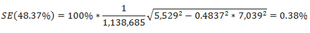
To calculate the lower and upper bounds of the 90 percent confidence interval around 48.37 using the standard error, simply multiply 0.38 by 1.645, then add and subtract the product from 48.37. Thus the 90 percent confidence interval for this estimate is [48.37 - 1.645(0.38)] to [48.37 + 1.645(0.38)], or 47.74% to 49.00%.
The estimate of the ratio is 587,937 / 550,748 = 1.068.Using formula (3) for the approximate standard error we have:
The 90 percent margin of error for this estimate would be 0.013 multiplied by 1.645, or about 0.021. The 90 percent lower and upper 90 percent confidence bounds would then be [1.068- 1.645(0.013)] to [1.068 + 1.645(0.013)], or 1.047 and 1.089.
SE(877,877) = 8,341/1.645= 5,071
and
SE(0.808) = 0.007/1.645 = 0.0042553
The approximate standard error for number of 1-unit detached owner-occupied housing units is calculated using formula (5) for products as:
To calculate the lower and upper bounds of the 90 percent confidence interval around 709,325 using the standard error, simply multiply 5,545 by 1.645, then add and subtract the product from 709,325. Thus the 90 percent confidence interval for this estimate is [709,325 - 1.645(5,545)] to [709,325 + 1.645(5,545)] or 700,203 to 718,447.
- Coverage Error
A major way to avoid coverage error in a survey is to ensure that its sampling frame, for Puerto Rico an address list in each municipio, is as complete and accurate as possible. The source of addresses for the PRCS is the MAF, which was created using the address list for Census 2000. An attempt is made to assign all appropriate geographic codes to each MAF address via an automated procedure using the Census Bureau TIGER (Topologically Integrated Geographic Encoding and Referencing) files. A manual coding operation based in the appropriate regional offices is attempted for addresses, which could not be automatically coded. The MAF was used as the source of addresses for selecting sample housing units and mailing questionnaires. TIGER produced the location maps for CAPI assignments. Sometimes the MAF has an address that is the duplicate of another address already on the MAF. This could occur when there is a slight difference in the address such as 123 Calle 1, Bayamon versus URB Hermosillo, 123 Calle 1, Bayamon.
In the CATI and CAPI nonresponse follow-up phases, efforts were made to minimize the chances that housing units that were not part of the sample were interviewed in place of units in sample by mistake. If a CATI interviewer called a mail nonresponse case and was not able to reach the exact address, no interview was conducted and the case was eligible for CAPI. During CAPI follow-up, the interviewer had to locate the exact address for each sample housing unit. If the interviewer could not locate the exact sample unit in a multi-unit structure, or found a different number of units than expected, the interviewers were instructed to list the units in the building and follow a specific procedure to select a replacement sample unit. Person overcoverage can occur when an individual is included as a member of a housing unit but does not meet PRCS residency rules.
Coverage rates give a measure of undercoverage or overcoverage of persons or housing units in a given geographic area. Rates below 100 percent indicate undercoverage, while rates above 100 percent indicate overcoverage. Coverage rates are released concurrent with the release of estimates on American FactFinder in the B98 series of detailed tables. Further information about PRCS coverage rates may be found at http://www.census.gov/acs/www/methodology/sample_size_and_data_quality/
- Nonresponse Error
- Unit Nonresponse - Unit nonresponse is the failure to obtain data from housing units in the sample. Unit nonresponse may occur because households are unwilling or unable to participate, or because an interviewer is unable to make contact with a housing unit. Unit nonresponse is problematic when there are systematic or variable differences between interviewed and noninterviewed housing units on the characteristics measured by the survey. Nonresponse bias is introduced into an estimate when differences are systematic, while nonresponse error for an estimate evolves from variable differences between interviewed and noninterviewed households.
The PRCS made every effort to minimize unit nonresponse, and thus, the potential for nonresponse error. First, the PRCS used a combination of mail, CATI, and CAPI data collection modes to maximize response. The mail phase included a series of three to four mailings to encourage housing units to return the questionnaire. Subsequently, mail nonrespondents (for which phone numbers are available) were contacted by CATI for an interview. Finally, a subsample of the mail and telephone nonrespondents was contacted for by personal visit to attempt an interview
PRCS response rates measure the percent of units with a completed interview. The higher the response rate, and consequently the lower the nonresponse rate, the less chance estimates may be affected by nonresponse bias. Response and nonresponse rates, as well as rates for specific types of nonresponse, are released concurrent with the release of estimates on American Factfinder in the B98 series of detailed tables. Further information about response and nonresponse rates may be found at http://www.census.gov/acs/www/methodology/sample_size_and_data_quality/.
- Item Nonresponse - Nonresponse to particular questions on the survey questionnaire and instrument allows for the introduction of error or bias into the data, since the characteristics of the nonrespondents have not been observed and may differ from those reported by respondents. As a result, any imputation procedure using respondent data may not completely reflect this difference either at the elemental level (individual person or housing unit) or on average.
Some protection against the introduction of large errors or biases is afforded by minimizing nonresponse. In the PRCS, item nonresponse for the CATI and CAPI operations was minimized by the requirement that the automated instrument receive a response to each question before the next one could be asked. Questionnaires returned by mail were edited for completeness and acceptability. They were reviewed by computer for content omissions and population coverage. If necessary, a telephone follow-up was made to obtain missing information. Potential coverage errors were included in this follow-up.
Allocation tables provide the weighted estimate of persons or housing units for which a value was imputed, as well as the total estimate of persons or housing units that were eligible to answer the question. The smaller the number of imputed responses, the lower the chance that the item nonresponse is contributing a bias to the estimates. Allocation tables are released concurrent with the release of estimates on American Factfinder in the B99 series of detailed tables with the overall allocation rates across all person and housing unit characteristics in the B98 series of detailed tables. Additional information on item nonresponse and allocations can be found at http://www.census.gov/acs/www/methodology/sample_size_and_data_quality/.
- Measurement and Processing Error
- Interviewer monitoring - The interviewer may misinterpret or otherwise incorrectly enter information given by a respondent; may fail to collect some of the information for a person or household; or may collect data for households that were not designated as part of the sample. To control these problems, the work of interviewers was monitored carefully. Field staff were prepared for their tasks by using specially developed training packages that included hands-on experience in using survey materials. A sample of the households interviewed by CAPI interviewers was reinterviewed to control for the possibility that interviewers may have fabricated data.
- Processing Error - The many phases involved in processing the survey data represent potential sources for the introduction of nonsampling error. The processing of the survey questionnaires includes the keying of data from completed questionnaires, automated clerical review, follow-up by telephone, manual coding of write-in responses, and automated data processing. The various field, coding and computer operations undergo a number of quality control checks to insure their accurate application.
- Content Editing - After data collection was completed, any remaining incomplete or inconsistent information was imputed during the final content edit of the collected data. Imputations, or computer assignments of acceptable codes in place of unacceptable entries or blanks, were needed most often when an entry for a given item was missing or when the information reported for a person or housing unit on that item was inconsistent with other information for that same person or housing unit. As in other surveys and previous censuses, the general procedure for changing unacceptable entries was to allocate an entry for a person or housing unit that was consistent with entries for persons or housing units with similar characteristics. Imputing acceptable values in place of blanks or unacceptable entries enhances the usefulness of the data.
A. Suppose we wish to estimate the total number of males with income below the poverty level in the past 12 months using both state and PUMA level estimates for the state of Wyoming. Part of the collapsed table C17001 is displayed below with estimates and their margins of error in parentheses.
Table A: 2009 Estimates of Males with Income Below Poverty from table C17001: Poverty Status in the Past 12 Months by Sex by Age
| Characteristic | Wyoming | PUMA 00100 | PUMA 00200 | PUMA 00300 | PUMA 00400 |
| Male | 23,001 (3,309) | 5,264 (1,624) | 6,508 (1,395) | 4,364 (1,026) | 6,865 (1,909) |
| Under 18 Years Old | 8,479 (1,874) | 2,041 (920) | 2,222 (778) | 1,999 (750) | 2,217 (1,192) |
| 18 to 64 Years Old | 12,976 (2,076) | 3,004 (1,049) | 3,725 (935) | 2,050 (635) | 4,197 (1,134) |
| 65 Years and Older | 1546 (500) | 219 (237) | 561 (286) | 315 (173) | 451 (302) |
| 2009 American FactFinder | |||||
The first way is to sum the three age groups for Wyoming:
Estimate(Male) = 8,479 + 12,976 + 1,546 = 23,001.
The first approximation for the standard error in this case gives us:
A second way is to sum the four PUMA estimates for Male to obtain:
Estimate(Male) = 5,264 + 6,508 + 4,364 + 6,865 = 23,001 as before.
The second approximation for the standard error yields:
Finally, we can sum up all three age groups for all four PUMAs to obtain an estimate based on a total of twelve estimates:
Estimate(Male) = 2,041 + 2,222 + ... + 451 = 23,001
And the third approximated standard error is
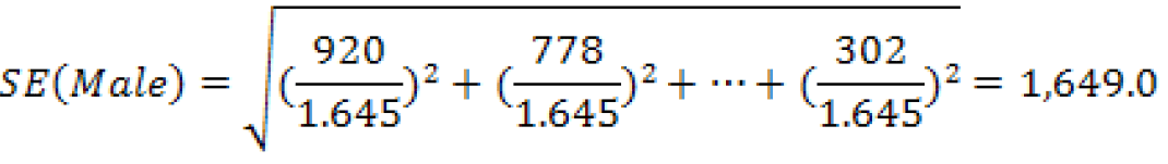
However, we do know that the standard error using the published MOE is 3,309 /1.645 = 2,011.6. In this instance, all of the approximations under-estimate the published standard error and should be used with caution.
B. Suppose we wish to estimate the total number of males at the national level using age and citizenship status. The relevant data from table B05003 is displayed in table B below.
Table B: 2009 Estimates of males from B05003: Sex by Age by Citizenship Status
| Characteristic | Estimate | MOE |
| Male | 151,375,321 | 27,279 |
| Under 18 Years | 38,146,514 | 24,365 |
| Native | 36,747,407 | 31,397 |
| Foreign Born | 1,399,107 | 20,177 |
| Naturalized U.S. Citizen | 268,445 | 10,289 |
| Not a U.S. Citizen | 1,130,662 | 20,228 |
| 18 Years and Older | 113,228,807 | 23,525 |
| Native | 95,384,433 | 70,210 |
| Foreign Born | 17,844,374 | 59,750 |
| Naturalized U.S. Citizen | 7,507,308 | 39,658 |
| Not a U.S. Citizen | 10,337,066 | 65,533 |
| 2009 American FactFinder | ||
The estimate and its MOE are actually published. However, if they were not available in the tables, one way of obtaining them would be to add together the number of males under 18 and over 18 to get:
Estimate (Male) = 38,146,514+ 113,223,807 = 151,375,321
And the first approximated standard error is
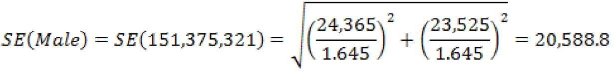
Another way would be to add up the estimates for the three subcategories (Native, and the two subcategories for Foreign Born: Naturalized U.S. Citizen, and Not a U.S. Citizen), for males under and over 18 years of age. From these six estimates we obtain:
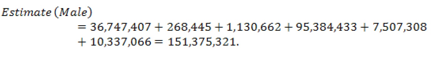
With a second approximated standard error of:
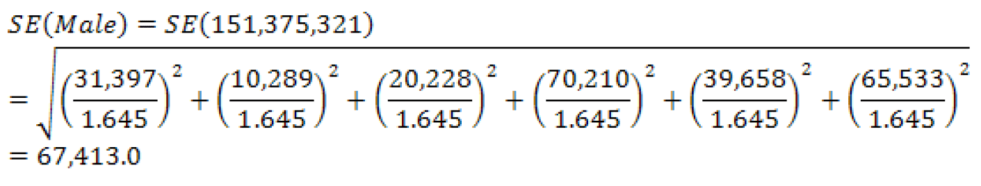
We do know that the standard error using the published margin of error is 27,279 / 1.645 = 16,583.0. With a quick glance, we can see that the ratio of the standard error of the first method to the published-based standard error yields 1.24; an over-estimate of roughly 24%, whereas the second method yields a ratio of 4.07 or an over-estimate of 307%. This is an example of what could happen to the approximate SE when the sum involves a controlled estimate. In this case, it is sex by age.
C. Suppose we are interested in the total number of people aged 65 or older and its standard error. Table C shows some of the estimates for the national level from table B01001 (the estimates in gray were derived for the purpose of this example only).
Table C: Some Estimates from AFF Table B01001: Sex by Age for 2009
| Age Category | Estimate, Male | MOE, Male | Estimate, Female | MOE, Female | Total | Estimated MOE, Total |
| 65 and 66 years old | 2,492,871 | 20,194 | 2,803,516 | 23,327 | 5,296,387 | 30,854 |
| 67 to 69 years old | 3,029,709 | 18,280 | 3,483,447 | 24,287 | 6,513,225 | 30,398 |
| 70 to 74 years old | 4,088,428 | 21,588 | 4,927,666 | 26,867 | 9,016,094 | 34,466 |
| 75 to 79 years old | 3,168,175 | 19,097 | 4,204,401 | 23,024 | 7,372,576 | 29,913 |
| 80 to 84 years old | 2,258,021 | 17,716 | 3,538,869 | 25,423 | 5,796,890 | 30,987 |
| 85 years and older | 1,743,971 | 17,991 | 3,767,574 | 19,294 | 5,511,545 | 26,381 |
| Total | 16,781,175 | NA | 22,725,473 | NA | 39,506,648 | 74,932 |
| 2009 American FactFinder | ||||||
To begin we find the total number of people aged 65 and over by simply adding the totals for males and females to get 16,781,175 + 22,725,542 = 39,506,717. One way we could use is summing males and female for each age category and then using their MOEs to approximate the standard error for the total number of people over 65.
... etc. ...
Now, we calculate for the number of people aged 65 or older to be 39,506,648 using the six derived estimates and approximate the standard error:
For this example the estimate and its MOE are published in table B09017. The total number of people aged 65 or older is 39,506,648 with a margin of error of 20,689. Therefore the published- based standard error is:
SE(39,506,643) = 20,689/1.645 = 12,577.
The approximated standard error, using six derived age group estimates, yields an approximated standard error roughly 3.6 times larger than the published-based standard error.
As a note, there are two additional ways to approximate the standard error of people aged 65 and over in addition to the way used above. The first is to find the published MOEs for the males age 65 and older and of females aged 65 and older separately and then combine to find the approximate standard error for the total. The second is to use all twelve of the published estimates together, that is, all estimates from the male age categories and female age categories, to create the SE for people aged 65 and older. However, in this particular example, the results from all three ways are the same. So no matter which way you use, you will obtain the same approximation for the SE. This is different from the results seen in example A.
D. For an alternative to approximating the standard error for people 65 years and older seen in part C, we could find the estimate and its SE by summing all of the estimate for the ages less than 65 years old and subtracting them from the estimate for the total population. Due to the large number of estimates, Table D does not show all of the age groups. In addition, the estimates in part of the table shaded gray were derived for the purposes of this example only and cannot be found in base table B01001.
Table D: Some Estimates from AFF Table B01001: Sex by Age for 2009:
| Age Category | Estimate, Male | MOE, Male | Estimate, Female | MOE, Female | Total | Estimated MOE, Total |
| Total Population | 151,375,321 | 27,279 | 155,631,235 | 27,280 | 307,006,556 | 38,579 |
| Under 5 years | 10,853,263 | 15,661 | 10,355,944 | 14,707 | 21,209,207 | 21,484 |
| 5 to 9 years old | 10,273,948 | 43,555 | 9,850,065 | 42,194 | 20,124,013 | 60,641 |
| 10 to 14 years old | 10,532,166 | 40,051 | 9,985,327 | 39,921 | 20,517,493 | 56,549 |
| ... | ... | ... | ... | ... | ||
| 62 to 64 years old | 4,282,178 | 25,636 | 4,669,376 | 28,769 | 8,951,554 | 38,534 |
| Total for Age 0 to 64 years old | 134,594,146 | 117,166 | 132,905,762 | 117,637 | 267,499,908 | 166,031 |
| Total for Age 65 years and older | 16,781,175 | 120,300 | 22,725,473 | 120,758 | 39,506,648 | 170,454 |
| 2009 American FactFinder | ||||||
An estimate for the number of people age 65 and older is equal to the total population minus the population between the ages of zero and 64 years old:
Number of people aged 65 and older: 307,006,556 - 267,499,908 = 39,506,648.
The way to approximate the SE is the same as in part C. First we will sum male and female estimates across each age category and then approximate the MOEs. We will use that information to approximate the standard error for our estimate of interest:
... etc. ...
And the SE for the total number of people aged 65 and older is:
Again, as in Example C, the estimate and its MOE are we published in B09017. The total number of people aged 65 or older is 39,506,648 with a margin of error of 20,689. Therefore the standard error is:
SE(39,506,648) = 20,689 / 1.645 = 12,577.
The approximated standard error using the thirteen derived age group estimates yields a standard error roughly 8.2 times larger than the actual SE.
Data users can mitigate the problems shown in examples A through D to some extent by utilizing a collapsed version of a detailed table (if it is available) which will reduce the number of estimates used in the approximation. These issues may also be avoided by creating estimates and SEs using the Public Use Microdata Sample (PUMS) or by requesting a custom tabulation, a fee- based service offered under certain conditions by the Census Bureau. More information regarding custom tabulations may be found at http://www.census.gov/acs/www/data_documentation/custom_tabulations/.

