


| Documentation: | Community Resilience Estimates |
you are here:
choose a survey
survey
document
chapter
Publisher: Community Resilience Estimates; Social, Economic, and Housing Statistics Division; U.S. Census Bureau
Survey: Community Resilience Estimates
| Document: | Community Resilience Estimate |
| citation: | Community Resilience Estimates; Social, Economic, and Housing Statistics Division; U.S. Census Bureau |
Chapter Contents

Define 2 nested high-level estimation layers (b-layers within a-layers) for parameter estimation and calibration. Nationwide, a-layer is defined as 9 divisions crossed with 4 urbanization strata, and the b-layers are 4-15 subsets within each a, mostly defined along CBSA boundaries.
Each a-layer is large enough so that parameter estimates, and resulting synthetic estimates, are negligibly correlated with tract-level ACS estimates.
Marginal post stratification estimates
For each a-layer-domain-risk component, edge rates are calculated.
These rates are applied to the tract-level population estimates by domain.
For each a-layer-domain-risk component, edge rates are calculated.
These rates are applied to the tract-level population estimates by domain.
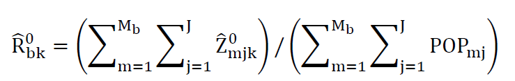
An adjustment is applied to the b-layer estimates that result from aggregating the post-stratified tract-level estimates across tracts and demographic groups.
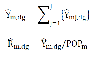
B-layer aggregates of the synthetic estimate across all demographic groups and resulting aggregate rates, and the corresponding direct estimate, 
 and resulting aggregate rates, and the corresponding direct estimate, are constructed.
The adjustment is calculated separately for each of the 36 a--layers, as un-weighted regression across the nested b-layers. Without the addition of further auxiliary data, this adjustment reduces to an intercept term. In other words it represents the difference in average rates between the initial post-stratified estimate and the ACS estimate.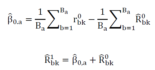
This mean adjustment can be larger than some of the 20 demographic-level post-stratification rates, Rather than apply
 at the tract-level, a raking factor is calculated for each b-layer. This raking is then applied to the initial tract-level count.
Regressions were designed at this high level of aggregation to avoid the prevalence of zeros at the tract-level, and maintain negligible correlation between synthetic and direct estimates at the tract level.
and resulting aggregate rates, and the corresponding direct estimate, are constructed.
The adjustment is calculated separately for each of the 36 a--layers, as un-weighted regression across the nested b-layers. Without the addition of further auxiliary data, this adjustment reduces to an intercept term. In other words it represents the difference in average rates between the initial post-stratified estimate and the ACS estimate.
This mean adjustment can be larger than some of the 20 demographic-level post-stratification rates,
Rather than apply
at the tract-level, a raking factor is calculated for each b-layer. This raking is then applied to the initial tract-level count.
Regressions were designed at this high level of aggregation to avoid the prevalence of zeros at the tract-level, and maintain negligible correlation between synthetic and direct estimates at the tract level.
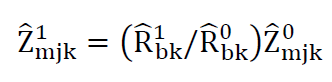
For a given risk component k*, ACS weighted aggregates are used at the a level to calculate the post-stratification ratios for the 64 permutations (both k*=0 and k*=1 outcomes) of all other risk components. For. The result is two 64 by 1 empirical probability vectors, conditional on the k* value,
 Apply these ratio vectors to the counts obtained in part 2.b. above.

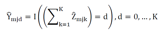
This results in a database of 128 by 20 age by rh groups by tract. This is repeated for all 7 of the dependent risk components. The final indirect estimate is the average of the 7 conditional estimates for each 128 by 20 age by rh groups by tract, thus
Apply these ratio vectors to the counts obtained in part 2.b. above.This results in a database of 128 by 20 age by rh groups by tract. This is repeated for all 7 of the dependent risk components. The final indirect estimate is the average of the 7 conditional estimates for each 128 by 20 age by rh groups by tract, thus
The target concept is an aggregate of individuals by the number of risk factors, categorized into 3 groups: zero flagged risk factors, one to two flagged risk factors, and three or more risk factors.
For the health risk factors, the proportions for each domain (region by age group by sex by rh group) is obtained from published NHIS tables.
The first step is to reduce the database size by summing across risk factor categories. For the target concept we are only considering the number of risk factors faced.
We split the resulting database by sex, as there are substantial differences in health risks by sex. The split uses the estimated population ratio of the sex in each age-race-ethnicity group, effectively setting the proportions for each of the prior risk factor groups equal between the sexes.
The proportions derived from NHIS tables are then applied to each domain, boosting the counts for higher risk numbers in each domain. This is repeated sequentially for each health condition.
The database size is further reduced by categorizing the RF-number by the 3 groups defined above.

We aggregate by tract forming these counts and rates.
For the health risk factors, the proportions for each domain (region by age group by sex by rh group) is obtained from published NHIS tables.
The first step is to reduce the database size by summing across risk factor categories. For the target concept we are only considering the number of risk factors faced.
We split the resulting database by sex, as there are substantial differences in health risks by sex. The split uses the estimated population ratio of the sex in each age-race-ethnicity group, effectively setting the proportions for each of the prior risk factor groups equal between the sexes.
The proportions derived from NHIS tables are then applied to each domain, boosting the counts for higher risk numbers in each domain. This is repeated sequentially for each health condition.
The database size is further reduced by categorizing the RF-number by the 3 groups defined above.
We aggregate by tract forming these counts and rates.
For the synthetic uncertainty estimate, we use a mean squared error approach relative to the average ACS sampling variance.
For the basic unweighted MoM estimator, and arbitrary collection of tracts, h, the equation is:

We use the following parameterization strategy. Assume the MSE for a given RF-group proportion estimate, is proportional to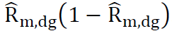
 is proportional to And that the constant of proportionality can be assumed stable over a wide range of RF-groups and tracts. Under the assumption of stability of the multiplicative constant, calculate this constant at an aggregate level, averaging across both RF-groups and tracts.
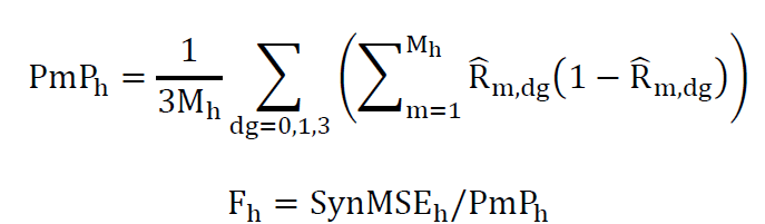
Under this strategy, modify the previous MoM equation to average across RF-groups as well as tracts:

And calculate the estimated constant at this level of aggregation in two steps:
Then for an individual tract:

This parameterization provides smooth, and stable, estimates that also satisfy the implicit constraints of the multinomial structure.
For the basic unweighted MoM estimator, and arbitrary collection of tracts, h, the equation is:
We use the following parameterization strategy. Assume the MSE for a given RF-group proportion estimate, is proportional to
is proportional to And that the constant of proportionality can be assumed stable over a wide range of RF-groups and tracts. Under the assumption of stability of the multiplicative constant, calculate this constant at an aggregate level, averaging across both RF-groups and tracts.Under this strategy, modify the previous MoM equation to average across RF-groups as well as tracts:
And calculate the estimated constant at this level of aggregation in two steps:
Then for an individual tract:
This parameterization provides smooth, and stable, estimates that also satisfy the implicit constraints of the multinomial structure.
For two predictors of the same concept, a linear combination of the two, with the usual relative MSE weighting shown below, has approximate optimality if the covariance between the two is low relative to the individual MSE. This modeling strategy was designed to maintain low correlation.

For the synthetic variance estimation,  and subsequent composite estimator, we need a reliable sampling variance estimate. The GVF value was used for all shrinkage.
The basic GVF formula was:
Given un-weighted counts of ACS respondents within tract m, notated nm. Fm is estimated with the regression,

The regression was estimated for all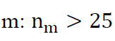
and subsequent composite estimator, we need a reliable sampling variance estimate. The GVF value was used for all shrinkage.The basic GVF formula was:
Given un-weighted counts of ACS respondents within tract m, notated nm. Fm is estimated with the regression,
The regression was estimated for all

