


| Documentation: | Census 2000 |
you are here:
choose a survey
survey
document
chapter
Publisher: U.S. Census Bureau
Survey: Census 2000
| Document: | Summary File 3 Technical Documentation |
| citation: | Social Explorer, U.S. Census Bureau; 2000 Census of Population and Housing, Summary File 3: Technical Documentation, 2002. |
Chapter Contents
User updates supply data users with additional or corrected information that becomes available after the technical documentation or files are prepared. They are issued as Count Question Resolution Notes, Data Notes, Geography Notes, and Technical Documentation Notes in a numbered series and are available in portable document format (PDF) on our Web site at http://www.census.gov.
If you print the documentation, please file the user updates cover sheet behind this notice. If there are technical documentation replacement pages, they should be filed in their proper location and the original pages destroyed.
If you print the documentation, please file the user updates cover sheet behind this notice. If there are technical documentation replacement pages, they should be filed in their proper location and the original pages destroyed.
On the Census 2000 long-form questionnaire, individuals could report more than one type of disability. Summary File 3 Table P41, Age by Types of Disability for the Civilian Noninstitutionalized Population 5 Years and Over With Disabilities, has as its universe the total disabilities tallied. Each line of the table represents the number of occurrences of a particular disability, and the numbers should be interpreted with care. For example, the second line of data in the table titled "Total disabilities tallied for people 5 to 15 years" does not refer to the number of people 5 to 15 years old, or to the number of people 5 to 15 with a disability. Rather it is the sum of the number of all disabilities reported among the 5 to 15 year old population. Lines in the table referencing specific disabilities are more easily interpreted. The third line in the table titled "Sensory disability," for example, refers to the number of sensory disabilities reported among people 5 to 15 years (or the number of people 5 to 15 years old with a sensory disability).
Data users wanting to know the percent of civilian noninstitutionalized people 5 to 15 years old with, for example, a sensory disability should divide line 3 from Table P41 with the sum of lines 3 and 27 from Table P42, Sex by Age by Disability Status by Employment Status for the Civilian Noninstitutionalized Population 5 Years and Over. Data users wanting to know the same percentages for one of the nine race or Hispanic or Latino origin groups should use Tables PCT67A-I and Tables PCT68A-I, as appropriate.
June 2002
Users may find slight differences in aggregate earnings for households between the Demographic Profile and Summary File 3 and related products. These differences are due to the treatment of offsetting positive and negative amounts for household members. Whenever offsetting values occurred, the Demographic Profile assigned these households a value zero while Summary File 3 and related products assigned a value of one dollar. The assignment of one dollar allows users to distinguish those households that had earnings from those households that did not have earnings. This will have little effect, if any, on mean household earnings.
June 2002
June 2002
Users may find slight differences in the Occupants Per Room calculations between the Demographic Profile and Summary File 3, Summary File 4, and related products. "Occupants per room" is obtained by dividing the number of people in each occupied housing unit by the number of rooms in the unit. The Summary File 3 products correctly used a top-code value of "10 rooms" for those occupied housing units with "9 or more rooms." In the Demographic Profiles, an incorrect top-code value of "9 rooms" was used.
June 2002
June 2002
In July 2002, the Census Bureau issued the following Data Note 4 regarding the Census 2000 Summary File 3 (SF3) data:
The Census Bureau is aware there may be a problem or problems in the employment-status data of Census 2000 Summary File 3 (including tables P38, P43-46, P149A-1, P150A-I, PCT35, PCT69A-1, and PCT 70A-1). The labor force data for some places where colleges are located appear to overstate the number in the labor force, the number unemployed, and the percent unemployed, probably because of reporting or processing errors. The exact cause is unknown, but the Census Bureau will continue to research the problem.
Our further research into this "college-town" issue indicates that the problem extended beyond places with colleges to the country in general. We learned that it stems from the tendency of many working-age people living in civilian noninstitutional group quarters (GQ), such as college dormitories, worker dormitories, and group homes (for the mentally ill or physically handicapped), to exhibit a particular pattern of entries to the employment questions in Census 2000.1 We now estimate that the pattern affected the employment data for about 15 percent of the civilian noninstitutional GQ population 16 years of age and over in the United States, or around 500,000 people. It had an impact on the Census 2000 labor force statistics for the entire country, but its effects were most visible and substantial for places, such as college towns, with high concentrations of people living in civilian noninstitutional group quarters.
In Census 2000, the majority of people in the GQ population were enumerated by the Individual Census Report (ICR) form, which collected employment data in a battery of six questions (questions 23, 27a-e). The responses to these questions were captured and fed into a set of rules (called the Employment Status Recode (ESR) edit) that used the combined information from all six questions to assign each person to one of the following four employment-status categories: not in universe (all people less than 16 years old), employed, unemployed, and not in labor force.
For a significant segment of the GQ population, a so-called "3/3" response pattern was entered into the ESR edit.2 This pattern is shown in the following table:
1The pattern also appeared frequently for people in institutional group quarters, such as prisons and juvenile institutions, but because of the way employment categories are defined, it had no impact on the employment data for these people.
2"3/3" refers to the fact that the responses to the first three questions, which appeared on page 4 of the ICR, are all missing; and those responses to the last three questions, which were on page 5 of the ICR, are all "yes."
The 3/3 pattern represents an incomplete set of information, since entries to the first three questions are missing. The ESR edit assigned people with this pattern to the unemployed category, because the edit had three built-in assumptions:
1) The respondents saw and reacted to each and every question in the employment series;
2) The 3/3 pattern represented the faithful recording of actual responses (or non-responses) to the questions; and
3) People who responded in this manner were more likely to meet the official criteria for the unemployed category than for any other category.3
Our research has revealed that most of the GQ cases with the 3/3 pattern may not have met one of the first two assumptions. We are still investigating, but we think that, in most cases, the pattern resulted from anomalies in the data collection or processing systems. Unfortunately, we cannot test our hypothesis by comparing the 3/3 pattern with actual reports from the respondents. The images of the filled-out ICRs will not be accessible until the completion, in 2006 at the earliest, of the Census Bureau's project to image the forms for delivery to the National Archives.
The potential effect of the ESR outcome for the 3/3 pattern is to increase the count of unemployed people at the expense of the counts of the employed and the not-in-labor-force groups. We have done some research to estimate the potential impact of the phenomenon on the labor force data for the nation as a whole. Our preliminary estimates are that it may have incorrectly decreased the number of employed people by about 235,000 (the number of employed in SF3 was 129.7 million), reduced the number of people not in the labor force by 285,000 (SF3 figure of 78.3 million), increased the number of unemployed by 519,000 (SF3 figure of 7.9 million), and raised the unemployment rate by 0.4 percentage point (SF3 figure was 5.8 percent).
Comparatively, the impact of the phenomenon on areas below the national level may be much greater, depending upon the relative size of the GQ population within the given area. The Census 2000 unemployment rate for the city of Williamsburg, Virginia, for example, was 41.7 percent (our research indicated that this rate resulted primarily from the prevalence of the 3/3 pattern among residents of college dormitories, who make up a large percentage of the city's population). To help data users gauge the impact of the phenomenon on their applications, and possibly to adjust for it, the Census Bureau released a tabulation of employment-status data for the nation, states, counties, and places, that was restricted to the population residing in households. This tabulation is available at: http://www.census.gov/hhes/www/laborfor.html
We will continue our research and report on further findings as they become available.
June 2004
3They reported that they were looking for work and could have started a job last week. Because they did not report whether they had a job last week (people with a job are classified as employed), it is reasonable to classify them as unemployed.
The Census Bureau is aware there may be a problem or problems in the employment-status data of Census 2000 Summary File 3 (including tables P38, P43-46, P149A-1, P150A-I, PCT35, PCT69A-1, and PCT 70A-1). The labor force data for some places where colleges are located appear to overstate the number in the labor force, the number unemployed, and the percent unemployed, probably because of reporting or processing errors. The exact cause is unknown, but the Census Bureau will continue to research the problem.
Our further research into this "college-town" issue indicates that the problem extended beyond places with colleges to the country in general. We learned that it stems from the tendency of many working-age people living in civilian noninstitutional group quarters (GQ), such as college dormitories, worker dormitories, and group homes (for the mentally ill or physically handicapped), to exhibit a particular pattern of entries to the employment questions in Census 2000.1 We now estimate that the pattern affected the employment data for about 15 percent of the civilian noninstitutional GQ population 16 years of age and over in the United States, or around 500,000 people. It had an impact on the Census 2000 labor force statistics for the entire country, but its effects were most visible and substantial for places, such as college towns, with high concentrations of people living in civilian noninstitutional group quarters.
In Census 2000, the majority of people in the GQ population were enumerated by the Individual Census Report (ICR) form, which collected employment data in a battery of six questions (questions 23, 27a-e). The responses to these questions were captured and fed into a set of rules (called the Employment Status Recode (ESR) edit) that used the combined information from all six questions to assign each person to one of the following four employment-status categories: not in universe (all people less than 16 years old), employed, unemployed, and not in labor force.
For a significant segment of the GQ population, a so-called "3/3" response pattern was entered into the ESR edit.2 This pattern is shown in the following table:
| 3/3 Input Pattern From ICR Forms | ||
|---|---|---|
| Question numberon ICR | Question wording | Entry |
| 23 | LAST WEEK, did you do ANY work for either pay or profit? | Missing |
| 27a | LAST WEEK, were you on layoff from a job? | Missing |
| 27b | LAST WEEK, were you TEMPORARILY absent from a job or business? | Missing |
| 27c | (For people on layoff) Have you been informed that you will be recalled to work within the next 6 months OR been given a date to return to work? | Yes |
| 27d | Have you been looking for work during the last four weeks? | Yes |
| 27e | LAST WEEK, could you have started a job if offered one, or returned to work if recalled? | Yes |
Footnotes:
1The pattern also appeared frequently for people in institutional group quarters, such as prisons and juvenile institutions, but because of the way employment categories are defined, it had no impact on the employment data for these people.
2"3/3" refers to the fact that the responses to the first three questions, which appeared on page 4 of the ICR, are all missing; and those responses to the last three questions, which were on page 5 of the ICR, are all "yes."
The 3/3 pattern represents an incomplete set of information, since entries to the first three questions are missing. The ESR edit assigned people with this pattern to the unemployed category, because the edit had three built-in assumptions:
1) The respondents saw and reacted to each and every question in the employment series;
2) The 3/3 pattern represented the faithful recording of actual responses (or non-responses) to the questions; and
3) People who responded in this manner were more likely to meet the official criteria for the unemployed category than for any other category.3
Our research has revealed that most of the GQ cases with the 3/3 pattern may not have met one of the first two assumptions. We are still investigating, but we think that, in most cases, the pattern resulted from anomalies in the data collection or processing systems. Unfortunately, we cannot test our hypothesis by comparing the 3/3 pattern with actual reports from the respondents. The images of the filled-out ICRs will not be accessible until the completion, in 2006 at the earliest, of the Census Bureau's project to image the forms for delivery to the National Archives.
The potential effect of the ESR outcome for the 3/3 pattern is to increase the count of unemployed people at the expense of the counts of the employed and the not-in-labor-force groups. We have done some research to estimate the potential impact of the phenomenon on the labor force data for the nation as a whole. Our preliminary estimates are that it may have incorrectly decreased the number of employed people by about 235,000 (the number of employed in SF3 was 129.7 million), reduced the number of people not in the labor force by 285,000 (SF3 figure of 78.3 million), increased the number of unemployed by 519,000 (SF3 figure of 7.9 million), and raised the unemployment rate by 0.4 percentage point (SF3 figure was 5.8 percent).
Comparatively, the impact of the phenomenon on areas below the national level may be much greater, depending upon the relative size of the GQ population within the given area. The Census 2000 unemployment rate for the city of Williamsburg, Virginia, for example, was 41.7 percent (our research indicated that this rate resulted primarily from the prevalence of the 3/3 pattern among residents of college dormitories, who make up a large percentage of the city's population). To help data users gauge the impact of the phenomenon on their applications, and possibly to adjust for it, the Census Bureau released a tabulation of employment-status data for the nation, states, counties, and places, that was restricted to the population residing in households. This tabulation is available at: http://www.census.gov/hhes/www/laborfor.html
We will continue our research and report on further findings as they become available.
June 2004
Footnotes:
3They reported that they were looking for work and could have started a job last week. Because they did not report whether they had a job last week (people with a job are classified as employed), it is reasonable to classify them as unemployed.
In Summary File 3 (SF 3), data are not available for four tables when using the geographic component1 rural farm (geographic component 49). These tables are:
P3. 100-Percent Count of the Population
P4. Percent of the Population in Sample
H3. 100-Percent Count of Housing Units
H4. Percent of Housing Units in Sample by Occupancy Status
This is because these tables refer to a 100-percent count, and the concept of farm residence2 is defined based on answers available only on the sample (long-form) questionnaire. Tables P3, P4, H3, and H4 are zero-filled for the rural farm geographic component. Also zero-filled are fields for land area, water area, population count (100-percent), housing unit count (100-percent), and internal points (latitude and longitude) in the geographic header record3.
For the remaining tables in SF 3, characteristics data are available for the rural farm geographic component. In the SF 3 state-level files, the rural farm data are available for states (summary level4 040) and counties (summary level 050). In the SF 3 national file, these data are available for the United States (summary level 010), regions (020), divisions (030), and states (040).
This note applies to the following data products:
1Geographic components and their codes are listed in the Census 2000 Summary File 3 Technical Documentation in Chapter 7 (Data Dictionary, Footnote Section).
2Detailed explanations of subject characteristics are found in the Census 2000 Summary File 3 Technical Documentation in Appendix B (Definitions of Subject Characteristics).
3A description of the geographic header record is found in the Census 2000 Summary File 3 Technical Documentation in Chapter 2 (How to Use This File).
4Complete summary level information is in the Census 2000 Summary File 3 Technical Documentation in Chapter 4 (Summary Level Sequence Chart).
P3. 100-Percent Count of the Population
P4. Percent of the Population in Sample
H3. 100-Percent Count of Housing Units
H4. Percent of Housing Units in Sample by Occupancy Status
This is because these tables refer to a 100-percent count, and the concept of farm residence2 is defined based on answers available only on the sample (long-form) questionnaire. Tables P3, P4, H3, and H4 are zero-filled for the rural farm geographic component. Also zero-filled are fields for land area, water area, population count (100-percent), housing unit count (100-percent), and internal points (latitude and longitude) in the geographic header record3.
For the remaining tables in SF 3, characteristics data are available for the rural farm geographic component. In the SF 3 state-level files, the rural farm data are available for states (summary level4 040) and counties (summary level 050). In the SF 3 national file, these data are available for the United States (summary level 010), regions (020), divisions (030), and states (040).
This note applies to the following data products:
- All SF 3 files available at the Census Bureau's FTP site.
- SF 3 CD-ROMs and DVDs.
- American FactFinder SF 3 detailed tables (geographic identifier for state geographic components)
Footnotes:
1Geographic components and their codes are listed in the Census 2000 Summary File 3 Technical Documentation in Chapter 7 (Data Dictionary, Footnote Section).
2Detailed explanations of subject characteristics are found in the Census 2000 Summary File 3 Technical Documentation in Appendix B (Definitions of Subject Characteristics).
3A description of the geographic header record is found in the Census 2000 Summary File 3 Technical Documentation in Chapter 2 (How to Use This File).
4Complete summary level information is in the Census 2000 Summary File 3 Technical Documentation in Chapter 4 (Summary Level Sequence Chart).
COMPARING SF 3 ESTIMATES WITH CORRESPONDING VALUES IN SF 1 AND SF 2
As in earlier censuses, the responses from the sample of households reporting on long forms must be weighted to reflect the entire population. Specifically, each responding household represents, on average, six or seven other households who reported using short forms.
One consequence of the weighting procedures is that each estimate based on the long form responses has an associated confidence interval. These confidence intervals are wider (as a percentage of the estimate) for geographic areas with smaller populations and for characteristics that occur less frequently in the area being examined (such as the proportion of people in poverty in a middle-income neighborhood).
In order to release as much useful information as possible, statisticians must balance a number of factors. In particular, for Census 2000, the Bureau of the Census created weighting areas-geographic areas from which about two hundred or more long forms were completed-which are large enough to produce good quality estimates. If smaller weighting areas had been used, the confidence intervals around the estimates would have been significantly wider, rendering many estimates less useful due to their lower reliability.
The disadvantage of using weighting areas this large is that, for smaller geographic areas within them, the estimates of characteristics that are also reported on the short form will not match the counts reported in SF 1 or SF 2. Examples of these characteristics are the total number of people, the number of people reporting specific racial categories, and the number of housing units. The official values for items reported on the short form come from SF 1 and SF 2.
The differences between the long form estimates in SF 3 and values in SF 1 or SF 2 are particularly noticeable for the smallest places, tracts, and block groups. The long form estimates of total population and total housing units in SF 3 will, however, match the SF 1 and SF 2 counts for larger geographic areas such as counties and states, and will be essentially the same for medium and large cities.
This phenomenon also occurred for the 1990 Census, although in that case, the weighting areas included relatively small places. As a result, the long form estimates matched the short form counts for those places, but the confidence intervals around the estimates of characteristics collected only on the long form were often significantly wider (as a percentage of the estimate).
SF 1 gives exact numbers even for very small groups and areas; whereas, SF 3 gives estimates for small groups and areas such as tracts and small places that are less exact. The goal of SF 3 is to identify large differences among areas or large changes over time. Estimates for small areas and small population groups often do exhibit large changes from one census to the next, so having the capability to measure them is worthwhile.
August 2002
The following new section was added to Chapter 8, Accuracy of the Data.
CONSISTENCY WITH COMPLETE COUNTS
As described earlier, Census 2000 long form data were collected on a sample basis. Cities and incorporated places were used to determine sampling rates to support estimates for these areas. As a result, each city, incorporated place, school district, and county had addresses selected in the long form sample.
To produce estimates from the long form data, weighting was performed at the weighting area level. In forming weighting areas, trade-offs between reliability, consistency of the estimates, and complexity of the implementation were considered. The decision was made to form weighting areas consisting of small geographic areas with at least 400 sample persons (or about 200 or more completed long forms) that do not cross county boundaries. No other boundary constraints were imposed. Thus, total population estimates from the long form data will agree with census counts reported in SF 1 and SF 2 for the weighting area, county, and other higher geographic areas obtained by combining either weighting areas or counties. Differences between long form estimates of characteristics in the SF 3 and their corresponding values in the SF 1 or SF 2 are particularly noticeable for small places, tracts, and block groups. Examples of these characteristics are the total number of people, the number of people reporting specific racial categories, and the number of housing units. The official values for items reported on the short form come from SF 1 and SF 2.
Because the weighting areas were formed at a smaller geographic level, any differential nonresponse to long form questionnaires by demographic groups or geographical areas included in a weighting area may introduce differences in complete counts (SF 1 and SF 2) and the SF 3 total population estimates. Also, an insufficient number of sample cases in the weighting matrix cells could lead to differences in SF 1, SF 2, and SF 3 population totals. Thus, differences between the census and SF 3 counts are typical and expected.
In 1990, separate tabulations were not prepared for small areas below a certain size. In contrast, Census 2000 tabulations are being prepared for all areas to maximize data availability. This approach may lead to a greater number of anomalous results than what may have been observed with tabulations released from the 1990 census. A similar phenomenon occurred in the 1990 census when weighting areas respected city and place boundaries. Census counts differed from the long form data estimates in small places. As expected, these differences were sometimes large.
The SF 1 tables provide the official census count of the number of people in an area. The SF 3 tables provide estimates of the proportion of people with specific characteristics, such as occupation, disability, or educational attainment. The total number of people in the SF 3 table is provided for use as the denominator, or base, for these proportions. Estimates in the SF 3 tables give the best estimates of the proportion of people with a particular characteristic, but the census count is the official count of how many people are in the area.
The SF 1 gives exact numbers even for very small groups and areas; whereas, SF 3 gives estimates for small groups and areas, such as tracts and small places, that are less exact. The goal of SF 3 is to identify large differences among areas or large changes over time. Estimates for small areas and small population groups often exhibit large changes from one census to the next, so having the capability to measure them is worthwhile.
August 2002
Median incomes for nonfamily households by race, Tables 156A through P156I, were calculated from a 38-category income distribution rather than the standard 39-category income distribution. The 38-category distribution collapsed the two highest categories ($175,000 - $199,999 and $200,000 and over) into a single category of $175,000 and over.
August 2002
August 2002
Census 2000 Summary File 3 CD-ROMs
Census 2000 Data Engine Software
Output | Create Output As Summary
The Census 2000 Summary File 3 database contains several tables of normalized data items, such as P53-Median Household Income in 1999, P82-Per Capita Income in 1999, and H18-Average Household Size of Occupied Housing Units by Tenure. In general, the Census 2000 Data Engine softwares Create Output As Summary function recognizes normalized data items and presents them as weighted averages of the summarized geographic components using the 100 percent population or housing count as the weighting factor. However, the version of the Census 2000 Data Engine software used on the Summary File 3 State CD-ROMs fails to recognize Per Capita as a one of the normalization techniques and performs a standard summation. This applies only to tables P82 and P157A through P157I. The Per Capita Income value displayed on the DP-3, Profile of Selected Economic Characteristics, is derived from the formula (P083001/P001001) rather than (P082001) as originally specified so that Create Output As Summary will perform correctly. The Summary File 3 DVD will contain a version of the software that performs a correct summation for Per Capita tables.
September 2002
The SF 3 table PCT55 data for "Nonfamily householders," nonfamily householders "Not living alone," and "Other unrelated individuals" have been removed. These data were removed because some respondents who were tallied as nonfamily householders "Not living alone" should have been tallied as "Other unrelated individuals." In American FactFinder, the data have been replaced with the symbol "(E)." In the files on the Census Bureau's FTP site, the data have been replaced with the value 999999999. The correct data will appear in SF 4 table PCT153.
February 2003
February 2003
FLORIDA
Summary File 3 state files for Florida contain missing data for the following three geographies:
88100US12349XX093,
88100US12349XX097, and
88100US12399XX111.
The Census Bureau has concluded that the three (3) geographies were tabulated with a result of Zero (0) population count and Zero (0) housing unit count and do not appear in the final summary file product.
This note is applicable to the following data products:
- Summary File 3 (SF 3) Florida state files available at the Census Bureau's FTP site.
- The Summary level is "State-5-digit ZCTA-County".
- SF 3 CD-ROMs (ASCII files only).
- Tables available on American FactFinder.
In Census 2000, during the conversion process of making the race write-in entries on the enumerator-filled questionnaire consistent with those in the mailout/mailback questionnaire, a step was inadvertently omitted. This resulted in an overstatement by about 1 million people reporting more than one race (or about 15 percent of the Two or More Races population). This overstatement almost entirely affects race combinations involving Some Other Race with the five race groups identified by the Office of Management and Budget (White, Black or African American, American Indian or Alaska Native, Asian, and Native Hawaiian or Other Pacific Islander). The overstatement does not significantly affect the totals for the Office of Management and Budget race groups reporting a single race (race alone) or the reporting of the single race and at least one other race (race alone or in combination).
March 2005
March 2005
| INDEX TO SUMMARY FILE 3 GEOGRAPHY NOTES | |
|---|---|
| Note | Geographic area |
| 1 | Alaska |
| 2 | California |
| 3 | Connecticut |
| 4 | Florida |
| 5 | Georgia |
| 6 | Nebraska |
| 7 | Tennessee |
| 8 | Wisconsin |
Alaska: 02
Nelson Lagoon Alaska Native village statistical area (ANVSA) (AIANHH 7025) erroneously contains block 2010, census tract 1 (000100) in Aleutians East census area (01598), Aleutians East Borough (013). This block should have not been coded to any ANVSA (9999). This is incorrect in both the PL 94-171 data products and Summary File (SF) data products.
This note applies to American FactFinder (AFF), CD-ROM, and redistricting data downloaded from the FTP site.
Internal Errata ID 02-003
May 2001Npar
California: 06
Los Angeles city (FIPS code 44000) erroneously contains block 1011, census tract 4002.03 (400203) in East San Gabriel Valley CCD (FIPS code 90810), Los Angeles County (FIPS code 037), CA (FIPS code 06). This block should have been coded to the place Balance of East San Gabriel Valley CCD (FIPS code 99999). This is incorrect in both the PL 94-171 data products and Summary File (SF) data products.
This note applies to American FactFinder (AFF), CD-ROM, and redistricting data downloaded from the FTP side.
Internal Errata ID 06-001
May 2001Lpar
Connecticut: 09
The place record, Balance of Milford town (FIPS code 99999) erroneously contains block 2999, census tract 1502 (150200) in Milford town (FIPS code 47535), New Haven County (FIPS code 009), CT (FIPS code 09). This block should have been coded to place Milford city (balance) (FIPS code 47515). This is incorrect in both the PL 94-171 data products and Summary File (SF) data products.
This note applies to American FactFinder (AFF), CD-ROM, and redistricting data downloaded from the FTP site.
Internal Errata ID 09-001
May 2001Tpar
Florida: 12
Yeehaw Junction CDP (FIPS code 78975) in St. Cloud CCD (FIPS code 93029), Osceola County (FIPS code 097), FL (FIPS code 12) should be named Buenaventura Lakes with FIPS code 09415. In 1990, this area was named Buena Ventura Lakes (FIPS code 09415). The area that should have been Yeehaw Junction CDP was erroneously not defined and does not appear in any Census 2000 products.
Internal Errata ID 12-001 May 2001
Georgia: 13
The place record Balance of Athens CCD (FIPS code 99999) erroneously contains blocks 2021 and 2023, census tract 1305 (130500) in Athens CCD (FIPS code 90138), Clarke County (FIPS code 059). Both blocks should have been coded to Bogart town (FIPS code 09068). The place record Balance of Winterville CCD (FIPS code 99999) erroneously contains blocks 1008 and 1009, census tract 1406 (140600) in Winterville CCD (93402), Clarke County (FIPS code 059). Both blocks should have been coded to the place Athens-Clarke County (balance) (FIPS code 03440). This is incorrect in both the PL 94-171 data products and Summary File (SF) data products.
This note applies to American FactFinder (AFF), CD-ROM, and redistricting data downloaded from the FTP site.
Internal Errata ID 13-001
May 2001Tpar
Nebraska: 31
In the PL 94-171 and Summary File (SF) data products, Cisco CDP (FIPS code 09112) in Lisco precinct (FIPS code 91790), Garden County (FIPS code 069), NE (FIPS code 31) should be named Lisco with FIPS code of 28315.
Internal Errata ID 31-002 May 2001
In the PL 94-171 and Summary File (SF) data products, Cisco CDP (FIPS code 09112) in Lisco precinct (FIPS code 91790), Garden County (FIPS code 069), NE (FIPS code 31) should be named Lisco with FIPS code of 28315.
Internal Errata ID 31-002 May 2001
Tennessee: 47
The place record Balance of Metropolitan Government CCD (FIPS code 99999) erroneously contains blocks 1001 and 1008, census tract 171 (017100) in Metropolitan Government CCD (FIPS code 92200), Davidson County (FIPS code 037), TN (FIPS code 47). Both blocks should have been coded to place Nashville-Davidson (balance) (FIPS code 52006). This is incorrect in both the PL 94-171 data products and Summary File (SF) data products.
Internal Errata ID 47-001
May 2001Tpar
Wisconsin: 55
The county subdivision of Scott town (FIPS code 72200), in place Balance of Scott town (FIPS code 99999) erroneously contains blocks 2048, 2063, and 2064, census tract 203 (020300), Brown County (FIPS code 009), WI (FIPS code 55). These blocks should have been coded to county subdivision and place Pulaski village (FIPS code 65675). The county subdivision of Pittsfield town (FIPS code 63075), in place Balance of Pittsfield town (FIPS code 99999) erroneously contains block 2049, census tract 203 (020300), Brown County (FIPS code 009). This block should have been coded to county subdivision and place Pulaski village (FIPS code 65675). This is incorrect in both the PL 94-171 data products and Summary File (SF) data products.
Internal Errata ID 55-001
May 2001Tpar
Chapter 8, Accuracy of the Data, was updated to reflect the fact that Tribal jurisdiction statistical areas were replaced for Census 2000 by entities called Oklahoma Tribal Statistical Areas.
October 2002
October 2002
Value, Price Asked was erroneously omitted from the list of aggregates subject to rounding on page B-69. The technical documentation has been corrected.
October 2002
October 2002
Cell 3 of Table HCT35B, Kitchen Facilities (Black or African American Alone Householder) in Chapter 6 and Chapter 7 was corrected to read "Lacking complete kitchen facilities." instead of "Lacking complete plumbing facilities."
November 2002
November 2002
Table HCT6, Tenure by Year Structure Built by Units in Structure, on page 7-453 was corrected to read "Renter occupied-Con." instead of "Owner occupied-Con."
November 2002
November 2002
The indentation of the "Management of companies and enterprises:" line of the Industry code list found in Appendix G was changed so that it is aligned with the "Administrative and support and waste management services:" line.
January 2003
January 2003
In the Race section of the Code List appendix, the tribes with codes F49-F52 were incorrectly listed under the tribal grouping "Monacan." These tribes should have appeared under the tribal grouping "Mono" as shown below:
September 2003
| Monacan | |
|---|---|
| F48 | Monacan Indian Nation |
| Mono | |
| F49 | Mono |
| F50 | North Fork Rancheria |
| F51 | Cold Springs Rancheria |
| F52 | Big Sandy Rancheria |
September 2003
The Language section of the Code List appendix had two spelling errors. They have been corrected to read as follows:
772 Tahitian
971 OTO-MANGUEAN
September 2003
772 Tahitian
971 OTO-MANGUEAN
September 2003
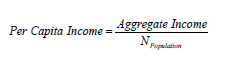
The Accuracy of the Data chapter describes how to calculate standard errors for most estimates, but not for per capita income, which is described below.
Per capita income is the total income from all sources (salary income, retirement income, public assistance income, etc.) of the people in a population group divided by the number of people in that group.
where N Population is the estimate of total people in the population group. A similar statistic, mean income, is like per capita income, except that the population measure includes only people at least 15 years of age, since income data is not collected for people younger than that.
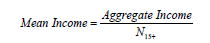
where N15+ is the estimate of people at least 15 years old in the population group.
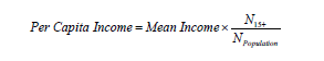
The two measures are related by the formula:
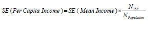
Hence, the approximate formula for estimating the standard error of per capita income is:
where N Population is the estimate of total people in the population group. A similar statistic, mean income, is like per capita income, except that the population measure includes only people at least 15 years of age, since income data is not collected for people younger than that.
where N15+ is the estimate of people at least 15 years old in the population group.
The two measures are related by the formula:
Hence, the approximate formula for estimating the standard error of per capita income is:
Calculating the standard error of Mean Income requires the use of an income distribution table. The table must provide frequency estimates of the number of people that fall within certain intervals. Standard available tables may be broken down by sex and whether the individual worked full-time, year-round in 1999. Such a table might look like this: U.S. Census Bureau, Census 2000.
Table 1. Sex by Work Experience in 1999 by Income in 1999 for the Population 15 Years and Over - Universe: Population 15 Years and Over
Following the distribution for Male: Worked Full-Time, Year-Round in 1999 (Wftyr) is a similar distribution for males who did not work full-time, year-round in 1999 (called Other in the table) and then females who did and did not work full-time, year-round in 1999.
1. To get the distribution of all people 15 years and older in each income interval, sum the four sex by work-status distributions:
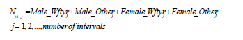
2. Sum the frequencies across all intervals j to obtain an estimate of the population total:

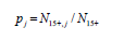
3. Calculate the estimated proportion of people in each income interval:
4. Calculate the mid-point (m) of each income interval from:

where Lj and Uj are the lower and upper bounds of the interval. If the cth interval is openended (i.e. has no upper bound), then an approximate value for mc is:

5. Estimate mean income from:

6. Estimate the standard error of mean income from:
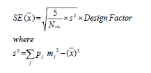
Use the design factor for Population: Household Income in 1999.
7. An approximation of per capita income can be computed by:

8. Multiply the result of Step 6 by the ratio of the person estimates

to get the approximate standard error for per capita income.
Example
This example shows the steps to estimate the standard error of per capita income for a population group in County A. 1. Sum the frequency estimates in each interval in the four sub-tables of Table 1 to produce a distribution similar to Table 2.
2. Cumulate the frequencies over the 21 intervals for those with and without income, to get the population base (N15+) of 32,091 people age 15 years and over.
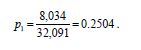
3. Calculate the proportion of people in each interval by dividing the intervals population estimate by the population base. The proportion of people age 15 and over in the No Income interval, p1, is
4. Find the midpoint mj for each of the 21 intervals.
For example, the midpoint of interval 3, $2,500 to $4,999 is
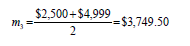
while the midpoint of the 21st interval, $100,000 or more is

The midpoint of the No Income interval is zero; for $1 to $2,499 or loss it is $1,250. Necessary results for the standard error calculation are given in Table 3 along with totals.
5. To estimate mean income of people at least 15 years old in the population group in County A, multiply each intervals proportion by its midpoint and sum over all intervals in the universe. Table 3 shows an estimated mean income of people at least 15 years, x , of $22,013
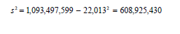
6. To estimate the standard error of mean income, first calculate the estimated population variance for mean income of people 15 years and older.
Suppose the person observed sampling rate in County A is 14.5 percent. Suppose the design factor for Population Household Income in 1999, given in the Less than 15 percent percent-in-sample column of the design factor table in the technical documentation, is 1.4. Use this information and the above results to calculate an estimated standard error for the mean income of people 15 years and older as:
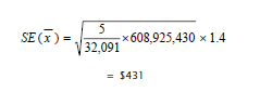
Thus the standard error on the mean income of $22,013 is $431.
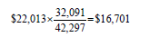
7. If the total population (including those less than 15 years old) in the population group in County A is 42,297, an approximation to per capita income is:
8. The standard error of the per capita income is calculated as:
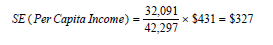
Thus the standard error of the per capita income of $16,701 is $327.
March 2004
Table 1. Sex by Work Experience in 1999 by Income in 1999 for the Population 15 Years and Over - Universe: Population 15 Years and Over
| Table 1. Sex by Work Experience in 1999 by Income in 1999 for the Population 15 Years and Over - Universe: Population 15 Years and Over | |
|---|---|
| Total | 32,091 |
| Male | 15,836 |
| Worked full-time, year-round in 1999: | 6,000 |
| No income | 0 |
| With income: | 6,000 |
| $1 to $2,499 or loss | 10 |
| $2,500 to $4,999 | 16 |
| $5,000 to $7,499 | 44 |
| $7,500 to $9,999 | 84 |
| . | |
| . | |
| . | |
| $100,000 or more | 146 |
Following the distribution for Male: Worked Full-Time, Year-Round in 1999 (Wftyr) is a similar distribution for males who did not work full-time, year-round in 1999 (called Other in the table) and then females who did and did not work full-time, year-round in 1999.
1. To get the distribution of all people 15 years and older in each income interval, sum the four sex by work-status distributions:
2. Sum the frequencies across all intervals j to obtain an estimate of the population total:
3. Calculate the estimated proportion of people in each income interval:
4. Calculate the mid-point (m) of each income interval from:
where Lj and Uj are the lower and upper bounds of the interval. If the cth interval is openended (i.e. has no upper bound), then an approximate value for mc is:
5. Estimate mean income from:
6. Estimate the standard error of mean income from:
Use the design factor for Population: Household Income in 1999.
7. An approximation of per capita income can be computed by:
8. Multiply the result of Step 6 by the ratio of the person estimates
to get the approximate standard error for per capita income.
Example
This example shows the steps to estimate the standard error of per capita income for a population group in County A. 1. Sum the frequency estimates in each interval in the four sub-tables of Table 1 to produce a distribution similar to Table 2.
| Table 2. Frequency Distribution for Income, People 15 years and older | |
|---|---|
| Total Income in 1999 | Frequency |
| No income | 8,034 |
| With income: | |
| $1 to $2,499 or loss | 644 |
| $2,500 to $4,999 | 730 |
| $5,000 to $7,499 | 876 |
| $7,500 to $9,999 | 1,299 |
| $10,000 to $12,499 | 1,350 |
| $12,500 to $14,999 | 1,438 |
| $15,000 to $17,499 | 1,599 |
| $17,500 to $19,999 | 1,688 |
| $20,000 to $22,499 | 1,871 |
| $22,500 to $24,999 | 1,766 |
| $25,000 to $29,999 | 2,331 |
| $30,000 to $34,999 | 1,923 |
| $35,000 to $39,999 | 1,345 |
| $40,000 to $44,999 | 914 |
| $45,000 to $49,999 | 856 |
| $50,000 to $54,999 | 1,134 |
| $55,000 to $64,999 | 828 |
| $65,000 to $74,999 | 563 |
| $75,000 to $99,999 | 455 |
| $100,000 or more | 447 |
| Total | 32,091 |
2. Cumulate the frequencies over the 21 intervals for those with and without income, to get the population base (N15+) of 32,091 people age 15 years and over.
3. Calculate the proportion of people in each interval by dividing the intervals population estimate by the population base. The proportion of people age 15 and over in the No Income interval, p1, is
4. Find the midpoint mj for each of the 21 intervals.
For example, the midpoint of interval 3, $2,500 to $4,999 is
while the midpoint of the 21st interval, $100,000 or more is
The midpoint of the No Income interval is zero; for $1 to $2,499 or loss it is $1,250. Necessary results for the standard error calculation are given in Table 3 along with totals.
| Table 3. Calculations for Per Capita Income | ||||
|---|---|---|---|---|
| Total Income in 1999 | pj | mj | pjmj2 | pjmj |
| No Income | 2504 | $0 | $0 | $0 |
| With Income | ||||
| $1 to $2,499 or loss | 201 | $125,000 | $31,406 | $2,513 |
| $2,500 to $4,999 | 227 | $374,950 | $319,134 | $8,511 |
| $5,000 to $7,499 | 273 | $624,950 | $1,066,236 | $17,061 |
| $7,500 to $9,999 | 405 | $874,950 | $3,100,427 | $35,435 |
| $10,000 to $12,499 | 421 | $1,124,950 | $5,327,808 | $47,360 |
| $12,500 to $14,999 | 448 | $1,374,950 | $8,469,384 | $61,598 |
| $15,000 to $17,499 | 498 | $1,624,950 | $13,149,503 | $80,923 |
| $17,500 to $19,999 | 526 | $1,874,950 | $18,491,201 | $98,622 |
| $20,000 to $22,499 | 583 | $2,124,950 | $26,324,855 | $123,885 |
| $22,500 to $24,999 | 550 | $2,374,950 | $31,022,131 | $130,622 |
| $25,000 to $29,999 | 726 | $2,749,950 | $54,901,754 | $199,646 |
| $30,000 to $34,999 | 599 | $3,249,950 | $63,267,428 | $194,672 |
| $35,000 to $39,999 | 419 | $3,749,950 | $58,920,304 | $157,123 |
| $40,000 to $44,999 | 285 | $4,249,950 | $51,476,914 | $121,124 |
| $45,000 to $49,999 | 267 | $4,749,950 | $60,240,607 | $126,824 |
| $50,000 to $54,999 | 353 | $5,249,950 | $97,293,772 | $185,323 |
| $55,000 to $64,999 | 258 | $5,999,950 | $92,878,452 | $154,799 |
| $65,000 to $74,999 | 175 | $6,999,950 | $85,748,775 | $122,499 |
| $75,000 to $99,999 | 142 | $8,749,950 | $108,717,508 | $124,249 |
| $100,000 or more | 139 | $15,000,000 | $312,750,000 | $208,500 |
| Total | $1,093,497,599 | $2,201,300 | ||
5. To estimate mean income of people at least 15 years old in the population group in County A, multiply each intervals proportion by its midpoint and sum over all intervals in the universe. Table 3 shows an estimated mean income of people at least 15 years, x , of $22,013
6. To estimate the standard error of mean income, first calculate the estimated population variance for mean income of people 15 years and older.
Suppose the person observed sampling rate in County A is 14.5 percent. Suppose the design factor for Population Household Income in 1999, given in the Less than 15 percent percent-in-sample column of the design factor table in the technical documentation, is 1.4. Use this information and the above results to calculate an estimated standard error for the mean income of people 15 years and older as:
Thus the standard error on the mean income of $22,013 is $431.
7. If the total population (including those less than 15 years old) in the population group in County A is 42,297, an approximation to per capita income is:
8. The standard error of the per capita income is calculated as:
Thus the standard error of the per capita income of $16,701 is $327.
March 2004

