


| Documentation: | Census 2000 |
you are here:
choose a survey
survey
document
chapter
Publisher: U.S. Census Bureau
Survey: Census 2000
| Document: | Summary File 3 Technical Documentation |
| citation: | Social Explorer, U.S. Census Bureau; 2000 Census of Population and Housing, Summary File 3: Technical Documentation, 2002. |
Chapter Contents
The data contained in this product are based on the Census 2000 sample. The data are estimates of the actual figures that would have been obtained from a complete count. Estimates derived from a sample are expected to be different from the 100-percent figures because they are subject to sampling and nonsampling errors. Sampling error in data arises from the selection of people and housing units included in the sample. Nonsampling error affects both sample and 100-percent data and is introduced as a result of errors that may occur during the data collection and processing phases of the census. This chapter provides a detailed discussion of both types of errors and a description of the estimation procedures.
The majority of addresses in the country are in what is known for census purposes as Mailout/Mailback areas, which generally consist of city-style addresses. The original source of addresses on the Master Address File (MAF) for the Mailout/Mailback areas was the 1990 Census Address Control File (ACF). The first update to the ACF addresses is a United States Postal Service (USPS) Delivery Sequence File (DSF) of addresses. The November 1997, September 1998, November 1999, and April 2000 DSFs were incorporated into the MAF.
Until shortly before the census, the ACF addresses and the November 1997 and September 1998 residential DSF addresses constituted the MAF. These addresses were tested against Census Bureau geographic information to determine their location at the census block level. The geographic information is maintained in the Census Bureau's Topologically Integrated Geographic Encoding Referencing (TIGER) system. When an address on the MAF can be uniquely matched to the address range in TIGER for a street segment that forms one of the boundaries of a particular block, the address is said to be geocoded to that block. Valid and geocoded addresses appeared on each address list used for a field operation.
The Block Canvass operation was the next major address list operation in the Mailout/Mailback areas for Census 2000. Between January and May 1999, there was a 100-percent canvass of every block in these areas. Every geocoded address was printed in a block-by-block address register. Block Canvassing listers identified each address as one of the following: a verified housing unit; a unit with corrections to the street name or directional; a delete; a duplicate, implying the unit exists elsewhere on the list with a different, unmatchable designation, such as a different street name or building name; uninhabitable; or nonresidential. Also, units that were deleted from one block and matched an added unit in another block were called a move.
A cooperative address list check with local governmental units throughout the country, called Local Update of Census Addresses (LUCA) 98, occurred in approximately the same time frame as Block Canvassing. In LUCA 98, the participating governmental units received an address list and were asked for input mostly on added units but also on deleted units and corrected street names or directionals. The outcome of this operation was similar to that of Block Canvassing; units were added to and deleted from blocks, and address corrections were made.
The Decennial Master Address File (DMAF), created in July 1999, was the file used for the main printing of the Census 2000 questionnaires. In Mailout/Mailback areas, the operations that had yielded housing units and their status before this initial printing stage were the ACF, the November 1997 DSF, the September 1998 DSF, LUCA 98, and Block Canvassing.
Updates to the DMAF followed the creation of the initial DMAF. Addresses were added by the November 1999, February 2000, and April 2000 DSFs. The LUCA 98 field verification and appeal processes were address update operations that occurred subsequent to the creation of the initial DMAF. Units receiving a conflicting status from Block Canvassing and the LUCA 98 operation were sent for field verification by the Census Bureau; the results of the field verification were sent to the governmental units. The governmental unit could appeal the Census Bureau's findings for particular units at this stage. At an appeal, the Census Bureau and the governmental unit submit their evidence of the status of a housing unit for independent review. The Census Address List Appeals Office, a temporary Federal office established outside the Department of Commerce, administered the appeal process. The Director of the Appeals Office (or their designee) was responsible for issuing a written determination that was considered final. Both the field verification and the appeal process had the potential to change the status of a housing unit.
The New Construction operation was another cooperative effort with participating governmental units that added addresses before Census Day. This was a final operation in Mailout/Mailback areas that used governmental units local knowledge to identify new housing units in February and March of 2000.
After Mailout/Mailback, the second most common method of questionnaire delivery was Update/Leave. Rather than obtaining addresses from the ACF and DSF, the address list for Update/Leave areas was constructed during a Census Bureau field operation called Address Listing. This was due to the fact that addresses in Update/Leave areas were primarily noncity-style. Census employees were sent to the field with maps of their assignment areas and were instructed to record the city-style address, noncity-style address or location description, or possibly some combination of the above, for every housing unit. In addition, the location of the unit was noted on the census map with what is known as a map spot . This operation took place in the fall of 1998.
After processing the Address Listing data, the Census Bureau could tabulate the number of housing units in each block. Because the housing units in these areas may have nonstandard mailing addresses and may be recorded in census files solely with a location description, the governmental units participating in the local review operation in these areas were sent lists of housing unit counts by block. This operation was called LUCA 99. When a LUCA 99 participant disagreed with a Census block count, the contested block was sent out for LUCA 99 recanvassing. Census employees were redeployed to make updates to the address list. In addition, there was a LUCA 99 appeal process for settling housing unit status discrepancies that could potentially add units to the address list. The LUCA 99 recanvassing and LUCA 99 appeal process took place at various times during the DMAF updating process. Although most of the LUCA 99 entities had their recanvassing results processed before creation of the initial DMAF, many did not. There were DMAF updates designed specifically for obtaining late recanvassing and appeal results. These updates to the census files occurred in time for USPS delivery of a questionnaire.
The last address list-building operation in the Update/Leave areas was the Update/Leave operation itself. This operation was responsible for having a census questionnaire hand-delivered at every housing unit. The MAF and the maps were updated during this process.
In the most remote regions of the country, housing units were listed at the same time people within them were enumerated for Census 2000. These operations, called List/Enumerate and Remote Alaska enumeration, were the only source of addresses in these regions. All housing units were map spotted at the time of enumeration.
In some other regions of the country where an address list had already been created, the Census Bureau determined that direct enumeration of the population would be more successful than mailback of the forms. This operation was called Update/Enumerate. There were two types of Update/Enumerate areas - urban areas that were formerly Mailout/Mailback and rural areas that were formerly Update/Leave. The urban areas had passed through all the Mailout/Mailback operations up through the point of the creation of the initial DMAF, and the rural areas had passed through Address Listing, and sometimes LUCA 99, by the time of the creation of the initial DMAF. Because of these distinct paths, it was necessary to distinguish between the urban and rural Update/Enumerate areas.
Urban Update/Leave is another special enumeration that took place in areas where mail delivery was considered to be problematic. The addresses had passed through all the operations of the Mailout/Mailback areas up through the creation of the initial DMAF, but enumerators visited the area during the census. As a result, additions, deletions and corrections to the address list were made.
People who do not receive a questionnaire at their house could submit a Be Counted Form, or they could call Telephone Questionnaire Assistance and have their information collected over the telephone. Addresses from these operations that did not match those already on the DMAF and that were geocoded to a census collection block in an area where census enumeration did not take place were visited in a Field Verification operation to determine if they existed. Verified addresses were added to the address list.
Follow-up operations provided additional information about housing units listed on the DMAF. In Nonresponse Followup (NRFU), enumerators followed up on units that had not returned a preaddressed census form. These units could be enumerated, deemed vacant, or possibly deleted. At the same time, units that did not appear on the address list could be added and enumerated concurrently. Coverage Improvement Follow Up was designated for enumeration at addresses added by New Construction and the later Delivery Sequence Files, as well as a second check on NRFU vacant and deleted units. Adds were also possible. These operations occurred in the Mailout/Mailback, Update/Leave, and Urban Update/Leave areas.
Service Based Enumeration was designed to account for people without a usual residence who use service facilities (i.e., shelters, soup kitchens and mobile food vans). Only people using the service facility on the interview day were enumerated. In addition, people enumerated in Targeted Non-Shelter Outdoor Locations (TNSOLS) and people without a usual residence that filed Be Counted Forms (BCF) augmented the count. This component of the enumeration should not be interpreted as a complete count of the population without a usual residence.
Every person and housing unit in the United States was asked basic demographic and housing questions (for example, race, age, and relationship to householder). A sample of these people and housing units was asked more detailed questions about items, such as income, occupation, and housing costs. The sampling unit for Census 2000 was the housing unit, including all occupants. There were four different housing unit sampling rates: 1-in-8, 1-in-6, 1-in-4, and 1-in-2 (designed for an overall average of about 1-in-6). The Census Bureau assigned these varying rates based on precensus occupied housing unit estimates of various geographic and statistical entities, such as incorporated places and interim census tracts. For people living in group quarters or enumerated at long form eligible service sites (shelters and soup kitchens), the sampling unit was the person and the sampling rate was 1-in-6.
The sample designation method for housing units depended on the data collection procedures. Approximately 95 percent of the population was enumerated by the mailback procedure. In these areas, the Census Bureau used the Decennial Master Address File (DMAF) to select electronically a probability sample. The questionnaires were either mailed or hand-delivered to selected addresses with instructions to complete and mail back the form.
The housing unit sampling rate varied by census block. Long Form Sampling Entities (LFSEs) were used to determine sampling rates in Census 2000 similarly to the way governmental units were used in the 1990 census sample design. LFSEs were:
In List/Enumerate areas (accounting for less than 0.5 percent of the housing units), each enumerator was given a blank address register with designated sample lines. Beginning about Census Day, the enumerator systematically canvassed an Assignment Area (AA) and listed all housing units in the address register in the order they were encountered. Completed questionnaires, including sample information for any housing unit listed on a designated sample line, were collected. If an AA contained any blocks that would qualify as above for a 1-in-2 or 1-in-4 rate, all households in the AA were sampled at 1-in-2. Housing units in all other AAs were sampled at 1-in-6.
Housing units in American Indian reservations, tribal jurisdiction statistical areas (replaced for Census 2000 by entities called Oklahoma Tribal Statistical Areas), and Alaska Native villages were sampled according to the same criteria as other LFSEs, except the sampling rates were based on the size of the American Indian and Alaska Native population in those areas as measured in the 1990 census. Trust lands were sampled at the highest rate of any part of their associated American Indian reservations. If the associated American Indian reservation was entirely outside the state containing the trust land, then the trust land was sampled at a 1-in-2 rate. All Remote Alaska assignment areas were sampled at a rate of 1-in-2. Housing units in Puerto Rico were sampled at a constant 1-in-6 rate in all blocks.
Variable sampling rates provide relatively more reliable estimates for small areas and decrease respondent burden in more densely populated areas while maintaining data reliability. When all sampling rates were taken into account across the Nation, approximately 1 out of every 6 housing units was included in the Census 2000 sample.
The sample designation method for housing units depended on the data collection procedures. Approximately 95 percent of the population was enumerated by the mailback procedure. In these areas, the Census Bureau used the Decennial Master Address File (DMAF) to select electronically a probability sample. The questionnaires were either mailed or hand-delivered to selected addresses with instructions to complete and mail back the form.
The housing unit sampling rate varied by census block. Long Form Sampling Entities (LFSEs) were used to determine sampling rates in Census 2000 similarly to the way governmental units were used in the 1990 census sample design. LFSEs were:
- Counties and county equivalents (such as parishes in Louisiana).
- Cities.
- Incorporated places (including consolidated cities).
- Census designated places in Hawaii only.
- Minor civil divisions in certain states only (Connecticut, Maine, Massachusetts, Michigan, Minnesota, New Hampshire, New Jersey, New York, Pennsylvania, Rhode Island, Vermont, and Wisconsin).
- School districts (based on the 1995-1996 school year).
- American Indian reservations.
- Tribal jurisdiction statistical areas (replaced for Census 2000 by entities called Oklahoma Tribal Statistical Areas).
- Alaska Native village statistical areas.
In List/Enumerate areas (accounting for less than 0.5 percent of the housing units), each enumerator was given a blank address register with designated sample lines. Beginning about Census Day, the enumerator systematically canvassed an Assignment Area (AA) and listed all housing units in the address register in the order they were encountered. Completed questionnaires, including sample information for any housing unit listed on a designated sample line, were collected. If an AA contained any blocks that would qualify as above for a 1-in-2 or 1-in-4 rate, all households in the AA were sampled at 1-in-2. Housing units in all other AAs were sampled at 1-in-6.
Housing units in American Indian reservations, tribal jurisdiction statistical areas (replaced for Census 2000 by entities called Oklahoma Tribal Statistical Areas), and Alaska Native villages were sampled according to the same criteria as other LFSEs, except the sampling rates were based on the size of the American Indian and Alaska Native population in those areas as measured in the 1990 census. Trust lands were sampled at the highest rate of any part of their associated American Indian reservations. If the associated American Indian reservation was entirely outside the state containing the trust land, then the trust land was sampled at a 1-in-2 rate. All Remote Alaska assignment areas were sampled at a rate of 1-in-2. Housing units in Puerto Rico were sampled at a constant 1-in-6 rate in all blocks.
Variable sampling rates provide relatively more reliable estimates for small areas and decrease respondent burden in more densely populated areas while maintaining data reliability. When all sampling rates were taken into account across the Nation, approximately 1 out of every 6 housing units was included in the Census 2000 sample.
The Census Bureau has modified or suppressed some data in this data release to protect confidentiality. Title 13 United States Code, Section 9, prohibits the Census Bureau from publishing results in which an individual can be identified. The Census Bureau's internal Disclosure Review Board sets the confidentiality rules for all data releases. A checklist approach is used to ensure that all potential risks to the confidentiality of the data are considered and addressed.
- Title 13, United States Code
- Disclosure limitation
- Data swapping
Statistics in this data product are based on a sample. Therefore, they may differ somewhat from 100-percent figures that would have been obtained if all housing units, people within those housing units, and people living in group quarters had been enumerated using the same questionnaires, instructions, enumerators, and so forth. The sample estimate also would differ from other samples of housing units, people within those housing units, and people living in group quarters. The deviation of a sample estimate from the average of all possible samples is called the sampling error . The standard error of a sample estimate is a measure of the variation among the estimates from all possible samples. Thus, it measures the precision with which an estimate from a particular sample approximates the average result of all possible samples. The sample estimate and its estimated standard error permit the construction of interval estimates with prescribed confidence that the interval includes the average result of all possible samples. The method of calculating standard errors and confidence intervals for the data in this product appears in the section called "Calculation of Standard Errors."
In addition to the variability that arises from the sampling procedures, both sample data and 100-percent data are subject to nonsampling error . Nonsampling error may be introduced during any of the various complex operations used to collect and process census data. For example, operations such as editing, reviewing, or handling questionnaires may introduce error into the data. A detailed discussion of the sources of nonsampling error is given in the section on "Nonsampling Error" in this chapter.
Nonsampling error may affect the data in two ways: errors that are introduced randomly will increase the variability of the data and, therefore, should be reflected in the standard error; errors that tend to be consistent in one direction will make both sample and 100-percent data biased in that direction. For example, if respondents consistently tend to underreport their incomes, then the resulting counts of households or families by income category will tend to be understated for the higher income categories and overstated for the lower income categories. Such biases are not reflected in the standard error.
By definition, universes that include the total population include both the household population and the group quarters population. For example, the universe defined as the population 15 years and over includes all people 15 years and over in both households and group quarters. In previous censuses and in Census 2000, allocation rates for demographic characteristics (such as age, sex, and race) of the group quarters population were similar to those for the total population. However, allocation rates for sample characteristics, such as school enrollment, educational attainment, income, and veteran status for the institutionalized and noninstitutionalized group quarters population have been substantially higher than those for the household population since at least the 1960 census. A review of the Census 2000 allocation rates for sample characteristics indicated that this trend continued.
Although allocation rates for sample characteristics are higher for the group quarters population, it is important to include the group quarters population in the total population universe. In most areas, the group quarters population represents a small proportion of the total population. As a result, the higher allocation rates associated with the group quarters population have minimal impact on the sample characteristics for the area of interest. In areas where the group quarters population represents a larger percentage of the total population, the Census Bureau cautions data users about the impact the higher allocation rates may have on the sample characteristics.
Although allocation rates for sample characteristics are higher for the group quarters population, it is important to include the group quarters population in the total population universe. In most areas, the group quarters population represents a small proportion of the total population. As a result, the higher allocation rates associated with the group quarters population have minimal impact on the sample characteristics for the area of interest. In areas where the group quarters population represents a larger percentage of the total population, the Census Bureau cautions data users about the impact the higher allocation rates may have on the sample characteristics.
Tables A through C in this chapter contain the necessary information for calculating the standard errors of sample estimates in this data product. To calculate the standard error, it is necessary to know:
Use the steps given below to calculate the standard error of an estimated total or percentage contained in this product. A percentage is defined here as a ratio of a numerator to a denominator where the numerator is a subset of the denominator. For example, the proportion of Black or African-American teachers is the ratio of Black or African-American teachers to all teachers.
1. Obtain the unadjusted standard error from Table A or B (or use the formula given below the table) for the estimated total or percentage, respectively.
2. Obtain the person or housing unit observed sampling rate (percent-in-sample) for the geographic area to which the estimate applies. Use the person observed sampling rate for population characteristics and the housing unit observed sampling rate for housing characteristics.
3. Use Table C to obtain the appropriate design factor, based on the characteristic (Employment status, School enrollment, etc.) and the range containing the percent-in-sample value defined in step 2. Multiply the unadjusted standard error by this design factor.
The unadjusted standard errors of zero estimates or of very small estimated totals or percentages will approach zero. This is also the case for very large percentages or estimated totals that are close to the size of the publication areas to which they correspond. Nevertheless, these estimated totals and percentages are still subject to sampling and nonsampling variability, and an estimated standard error of zero (or a very small standard error) is not appropriate. For estimated percentages that are less than 2 or greater than 98, use the unadjusted standard errors in Table B that appear in the "2 or 98" row. For an estimated total that is less than 50 or within 50 of the total size of the publication area, use an unadjusted standard error of 16.
Examples using Tables A and B are given in the section titled "Using Tables to Compute Standard Errors and Confidence Intervals."
- The unadjusted standard error for the characteristic (given in Table A for estimated totals or Table B for estimated percentages) that would result under a simple random sample design of people, housing units, households, or families.
- The design factor for the particular characteristic estimated (given in Table C) based on the sample design and estimation techniques employed to produce long form data estimates.
- The number of people, housing units, households, or families in the publication area.
- The observed sampling rate.
Use the steps given below to calculate the standard error of an estimated total or percentage contained in this product. A percentage is defined here as a ratio of a numerator to a denominator where the numerator is a subset of the denominator. For example, the proportion of Black or African-American teachers is the ratio of Black or African-American teachers to all teachers.
1. Obtain the unadjusted standard error from Table A or B (or use the formula given below the table) for the estimated total or percentage, respectively.
2. Obtain the person or housing unit observed sampling rate (percent-in-sample) for the geographic area to which the estimate applies. Use the person observed sampling rate for population characteristics and the housing unit observed sampling rate for housing characteristics.
3. Use Table C to obtain the appropriate design factor, based on the characteristic (Employment status, School enrollment, etc.) and the range containing the percent-in-sample value defined in step 2. Multiply the unadjusted standard error by this design factor.
The unadjusted standard errors of zero estimates or of very small estimated totals or percentages will approach zero. This is also the case for very large percentages or estimated totals that are close to the size of the publication areas to which they correspond. Nevertheless, these estimated totals and percentages are still subject to sampling and nonsampling variability, and an estimated standard error of zero (or a very small standard error) is not appropriate. For estimated percentages that are less than 2 or greater than 98, use the unadjusted standard errors in Table B that appear in the "2 or 98" row. For an estimated total that is less than 50 or within 50 of the total size of the publication area, use an unadjusted standard error of 16.
Examples using Tables A and B are given in the section titled "Using Tables to Compute Standard Errors and Confidence Intervals."
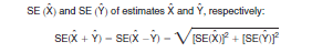
The standard errors estimated from Tables A and B are not directly applicable to sums of and differences between two sample estimates. To estimate the standard error of a sum or difference, the tables are to be used somewhat differently in the following three situations:
1. For the sum of or difference between a sample estimate and a 100-percent value, use the standard error of the sample estimate. The complete count value is not subject to sampling error.
2. For the sum of or difference between two sample estimates, the appropriate standard error is approximately the square root of the sum of the two individual standard errors squared; that is, for standard errors
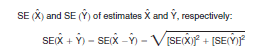
This method, however, will underestimate (overestimate) the standard error if the two items in a sum are highly positively (negatively) correlated or if the two items in a difference are highly negatively (positively) correlated. This method may also be used for the difference between (or sum of) sample estimates from two censuses or from a census sample and another survey. The standard error for estimates not based on the Census 2000 sample must be obtained from an appropriate source outside of this chapter. 3. For the differences between two estimates, one of which is a subclass of the other, use the tables directly where the calculated difference is the estimate of interest. For example, to determine the estimate of non-Black or African-American teachers, subtract the estimate of Black or African-American teachers from the estimate of total teachers. To determine the standard error of the estimate of non-Black or African-American teachers, apply the above formula directly.
1. For the sum of or difference between a sample estimate and a 100-percent value, use the standard error of the sample estimate. The complete count value is not subject to sampling error.
2. For the sum of or difference between two sample estimates, the appropriate standard error is approximately the square root of the sum of the two individual standard errors squared; that is, for standard errors
This method, however, will underestimate (overestimate) the standard error if the two items in a sum are highly positively (negatively) correlated or if the two items in a difference are highly negatively (positively) correlated. This method may also be used for the difference between (or sum of) sample estimates from two censuses or from a census sample and another survey. The standard error for estimates not based on the Census 2000 sample must be obtained from an appropriate source outside of this chapter. 3. For the differences between two estimates, one of which is a subclass of the other, use the tables directly where the calculated difference is the estimate of interest. For example, to determine the estimate of non-Black or African-American teachers, subtract the estimate of Black or African-American teachers from the estimate of total teachers. To determine the standard error of the estimate of non-Black or African-American teachers, apply the above formula directly.
Frequently, the statistic of interest is the ratio of two variables, where the numerator is not a subset of the denominator. An example is the ratio of students to teachers in public elementary schools. (Note that this method cannot be used to compute a standard error for a sample mean.) The standard error of the ratio between two sample estimates is estimated as follows:
1. If the ratio is a proportion, then follow the procedure outlined for "Totals and percentages."
2. If the ratio is not a proportion, then approximate the standard error using the formula below.
1. If the ratio is a proportion, then follow the procedure outlined for "Totals and percentages."
2. If the ratio is not a proportion, then approximate the standard error using the formula below.
The sampling variability of an estimated median depends on the form of the distribution and the size of its base. The reliability of an estimated median is approximated by constructing a confidence interval. Estimate the 68 percent confidence limits of a median based on sample data using the following procedure.
1. Obtain the appropriate (person or housing unit) observed sampling rate for the specific geographic area. Use this rate to locate the design factor for the characteristic of interest in Table C.
2. Obtain the frequency distribution for the selected variable. Cumulate these frequencies to yield the base.
3. Determine the standard error of the estimate of 50 percent from the distribution using the formula:

4. Subtract from and add to 50 percent the standard error determined in step 3.
p_lower = 50 -SE (50 percent)
p_upper = 50 + SE (50 percent)
Find the category in the distribution containing p_lower and the category in the distribution containing p_upper. If p_lower and p_upper fall in the same category, follow these steps:

where X = p_lower (p_upper)for the Lower Bound (Upper Bound).
6. Divide the difference between the two points determined in step 5 by two to obtain the estimated standard error of the median:

1. Obtain the appropriate (person or housing unit) observed sampling rate for the specific geographic area. Use this rate to locate the design factor for the characteristic of interest in Table C.
2. Obtain the frequency distribution for the selected variable. Cumulate these frequencies to yield the base.
3. Determine the standard error of the estimate of 50 percent from the distribution using the formula:
4. Subtract from and add to 50 percent the standard error determined in step 3.
p_lower = 50 -SE (50 percent)
p_upper = 50 + SE (50 percent)
Find the category in the distribution containing p_lower and the category in the distribution containing p_upper. If p_lower and p_upper fall in the same category, follow these steps:
- Define A1 as the smallest value in that category.
- Define A2 to be the smallest value in the next (higher) category.
- Define C1 as the cumulative percent of units strictly less than A1.
- Define C2 as the cumulative percent of units strictly less than A2.
- First, for the category containing p_lower, define the values A1, A2, C1, and C2 as above. Use these values in step 5 to obtain the Lower Bound.
- Second, for the category containing p_upper, define a new set of values for A1, A2, C1, and C2. Use these values in step 5 to obtain the Upper Bound.
where X = p_lower (p_upper)for the Lower Bound (Upper Bound).
6. Divide the difference between the two points determined in step 5 by two to obtain the estimated standard error of the median:
A mean is defined here as the average quantity of some characteristic (other than the number of people, housing units, households, or families) per person, housing unit, household, or family. For example, a mean could be the average annual income of females age 25 to 34. The standard error of a mean can be approximated by the formula below. Because of the approximation used in developing this formula, the estimated standard error of the mean obtained from this formula will generally underestimate the true standard error.
The formula for estimating the standard error of a mean, x , is
where s2 is the estimated population variance of the characteristic and the base is the total number of units in the population. The population variance, s2, may be estimated using data that has been grouped into intervals. For this method, the range of values for the characteristic is divided into c intervals, where the lower and upper boundaries of interval j are 'Lj' and 'Uj', respectively. Each person is placed into one of the c intervals such that the value of the characteristic is between 'Lj' and 'Uj'. The estimated population variance, s2, is then given by:

where pj is the estimated proportion of persons in interval j (based on weighted data) and mj is the midpoint of the jth interval, calculated as:

The most representative value of the characteristic in interval j is assumed to be the midpoint of the interval, mj. If the cth interval is open-ended, i.e., no upper interval boundary exists, then an approximate value for mc is

The estimated sample mean, x, can be obtained using the following formula:

The formula for estimating the standard error of a mean, x , is
where s2 is the estimated population variance of the characteristic and the base is the total number of units in the population. The population variance, s2, may be estimated using data that has been grouped into intervals. For this method, the range of values for the characteristic is divided into c intervals, where the lower and upper boundaries of interval j are 'Lj' and 'Uj', respectively. Each person is placed into one of the c intervals such that the value of the characteristic is between 'Lj' and 'Uj'. The estimated population variance, s2, is then given by:
where pj is the estimated proportion of persons in interval j (based on weighted data) and mj is the midpoint of the jth interval, calculated as:
The most representative value of the characteristic in interval j is assumed to be the midpoint of the interval, mj. If the cth interval is open-ended, i.e., no upper interval boundary exists, then an approximate value for mc is
The estimated sample mean, x, can be obtained using the following formula:
A sample estimate and its estimated standard error may be used to construct confidence intervals about the estimate. These intervals are ranges that will contain the average value of the estimated characteristic that results over all possible samples, with a known probability.
For example, if all possible samples that could result under the Census 2000 sample design were independently selected and surveyed under the same conditions, and if the estimate and its estimated standard error were calculated for each of these samples, then:
1. 68 percent confidence interval. Approximately 68 percent of the intervals from one estimated standard error below the estimate to one estimated standard error above the estimate would contain the average result from all possible samples.
2. 90 percent confidence interval. Approximately 90 percent of the intervals from 1.645 times the estimated standard error below the estimate to 1.645 times the estimated standard error above the estimate would contain the average result from all possible samples.
3. 95 percent confidence interval. Approximately 95 percent of the intervals from two estimated standard errors below the estimate to two estimated standard errors above the estimate would contain the average result from all possible samples.
The average value of the estimated characteristic that could be derived from all possible samples either is or is not contained in any particular computed interval. Thus, the statement that the average value has a certain probability of falling between the limits of the calculated confidence interval cannot be made. Rather, one can say with a specified probability of confidence that the calculated confidence interval includes the average estimate from all possible samples (approximately the 100-percent value).
Confidence intervals also may be constructed for the ratio, sum of, or difference between two sample figures. First compute the ratio, sum, or difference. Next, obtain the standard error of the ratio, sum, or difference (using the formulas given earlier). Finally, form a confidence interval for this estimated ratio, sum, or difference as above. One can then say with specified confidence that this interval includes the ratio, sum, or difference that would have been obtained by averaging the results from all possible samples.
To calculate the lower and upper bounds of the 90 percent confidence interval around an estimate using the standard error, multiply the standard error by 1.645, then add and subtract the product from the estimate.
Lower bound = Estimate - (Standard Error *1.645)
Upper bound = Estimate + (Standard Error * 1.645)
Lower bound = Estimate - (Standard Error *1.645)
Upper bound = Estimate + (Standard Error * 1.645)
Be careful when computing and interpreting confidence intervals. The estimated standard errors given in this chapter do not include all portions of the variability because of nonsampling error that may be present in the data. The standard errors reflect the effect of simple response variance, but not the effect of correlated errors introduced by enumerators, coders, or other field or processing personnel. Thus, the standard errors calculated represent a lower bound of the total error. As a result, confidence intervals formed using these estimated standard errors might not meet the stated levels of confidence (i.e., 68, 90, or 95 percent). Thus, be careful interpreting the data in this data product based on the estimated standard errors.
A standard sampling theory text should be helpful if the user needs more information about confidence intervals and nonsampling errors.
Zero or small estimates; very large estimates. The value of almost all Census 2000 characteristics is greater than or equal to zero by definition. The method given previously for calculating confidence intervals relies on large sample theory and may result in negative values for zero or small estimates, which are not admissible for most characteristics. In this case, the lower limit of the confidence interval is set to zero by default. A similar caution holds for estimates of totals that are close to the population total and for estimated proportions near one, where the upper limit of the confidence interval is set to its largest admissible value. In these situations, the level of confidence of the adjusted range of values is less than the prescribed confidence level.
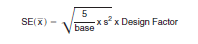
Suppose a particular data table shows that for City A 9,948 people out of all 15,888 people age 16 years and over were in the civilian labor force. The person observed sampling rate (percent-in-sample) in City A is 16.0 percent. The column in Table C that includes an observed sampling rate of 16.0 percent shows the design factor to be 1.1 for the population characteristic "Employment status."
The unadjusted standard error for the estimated total of 9,948 is computed using the formula given below Table A. Suppose that the total population of City A was 21,220. The formula for the unadjusted standard error, SE, is
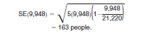
The 5 in the above formula is based on a 1-in-6 sample and is derived from the inverse of the sampling rate minus one; i.e., 5 = 6 x 1. To find the standard error of the estimated 9,948 people 16 years and over who were in the civilian labor force, multiply the unadjusted standard error 163 by the design factor, 1.1, from Table C. This yields an estimated standard error of 179 for the total number of people 16 years and over in City A who were in the civilian labor force.
The unadjusted standard error for the estimated total of 9,948 is computed using the formula given below Table A. Suppose that the total population of City A was 21,220. The formula for the unadjusted standard error, SE, is
The 5 in the above formula is based on a 1-in-6 sample and is derived from the inverse of the sampling rate minus one; i.e., 5 = 6 x 1. To find the standard error of the estimated 9,948 people 16 years and over who were in the civilian labor force, multiply the unadjusted standard error 163 by the design factor, 1.1, from Table C. This yields an estimated standard error of 179 for the total number of people 16 years and over in City A who were in the civilian labor force.
The estimated percent of people 16 years and over who were in the civilian labor force in City A is 62.6 percent (= 9,948 / 15,888). Using the formula below Table B, the unadjusted standard error is approximately

Again, the 5 in the above formula is based on a 1-in-6 sample and is derived from the inverse of the sampling rate minus one; i.e., 5 = 6 x 1. The standard error for the estimated 62.6 percent of people 16 years and over who were in the civilian labor force is 0.86 x 1.1 = 0.95 percentage points.
Note that standard errors of percentages derived in this manner are approximate. Calculations can be expressed to several decimal places, but doing so would indicate more precision in the data than is justifiable. Final results should contain no more than two decimal places when the estimated standard error is one percentage point (i.e., 1.00) or more.
In Example 1, the adjusted standard error of the 9,948 people 16 years and over in City A in the civilian labor force was 179. Thus, a 90 percent confidence interval for this estimated total is:
[9,948 - 1.645(179)] to [9,948 + 1.645 (179)] or 9,654 to 10,242.
One can say, with about 90 percent confidence, that this interval includes the value that would have been obtained by averaging the results from all possible samples.
[9,948 - 1.645(179)] to [9,948 + 1.645 (179)] or 9,654 to 10,242.
One can say, with about 90 percent confidence, that this interval includes the value that would have been obtained by averaging the results from all possible samples.
Suppose the number of people in City B age 16 years and over who were in the civilian labor force was 9,314 and the total number of people 16 years and over was 16,666. The population size of City B was 25,225, resulting in a person percent-in-sample of 15.7. The range that includes an observed sampling rate of 15.7 in Table C shows the design factor to be 1.1 for "Employment status." Using the formula below Table A and the appropriate design factor, the estimated standard error for the total number of people 16 years and over in City B who were in the civilian labor force is 188 (= 171 x 1.1). The estimated percentage of people 16 years and over who were in the civilian labor force is 55.9 percent. The unadjusted standard error determined using the formula provided at the bottom of Table B is 0.86 percentage points, and the approximate standard error of the percentage (55.9 percent) is 0.86 x 1.1 = 0.95 percentage points.
Suppose that one wished to obtain the standard error of the difference between City A and City B of the percentages of people who were 16 years and over and who were in the civilian labor force. The difference in the percentages for the two cities is:
62.6 - 55.9 = 6.7 percent.
Using the above calculations and the adjusted standard error from Example 2:
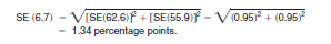
The 90 percent confidence interval for the difference is formed as before:
[6.70 - 1.645 (1.34)] to [6.70 + 1.645(1.34)] or 4.50 to 8.90.
One can say with 90 percent confidence that the interval includes the difference that would have been obtained by averaging the results from all possible samples.
Suppose that one wished to obtain the standard error of the difference between City A and City B of the percentages of people who were 16 years and over and who were in the civilian labor force. The difference in the percentages for the two cities is:
62.6 - 55.9 = 6.7 percent.
Using the above calculations and the adjusted standard error from Example 2:
The 90 percent confidence interval for the difference is formed as before:
[6.70 - 1.645 (1.34)] to [6.70 + 1.645(1.34)] or 4.50 to 8.90.
One can say with 90 percent confidence that the interval includes the difference that would have been obtained by averaging the results from all possible samples.
For reasonably large samples, ratio estimates are normally distributed, particularly for the census population. Therefore, if the standard error of a ratio estimate can be calculated, then a confidence interval can be formed about the ratio. Suppose that one wished to obtain the standard error of the ratio of the estimate of people who were 16 years and over and who were in the civilian labor force in City A to the estimate of people who were 16 years and over and who were in the civilian labor force in City B. The ratio of the two estimates is:
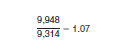
The standard error of this ratio is:
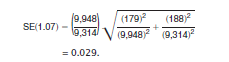
Using the results above, the 90 percent confidence interval for this ratio would be:
[1.07 - 1.645(0.029)] to [1.07 + 1.65(0.029)] or 1.02 to 1.12.
One can say with 90 percent confidence that the interval includes the ratio that would have been obtained by averaging the results from all possible samples.
The standard error of this ratio is:
Using the results above, the 90 percent confidence interval for this ratio would be:
[1.07 - 1.645(0.029)] to [1.07 + 1.65(0.029)] or 1.02 to 1.12.
One can say with 90 percent confidence that the interval includes the ratio that would have been obtained by averaging the results from all possible samples.
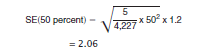
The following example shows the steps for calculating an estimated standard error and confidence interval for the median housing value in City C.
1. The housing unit observed sampling rate in City C is 14.3. Suppose that the corresponding design factor in Table C for the housing characteristic "Value" is 1.2.
2. Obtain the frequency distribution for housing values in City C. The base is the sum of the frequencies (4,227).
3. Determine the standard error of the estimate of 50 percent from the distribution:
4. Calculate a confidence interval with bounds:
p_lower =50 -2.06 = 47.94
p_upper = 50 - 2.06 = 52.06
From the given distribution, the category with the cumulative percent first exceeding 47.94 percent is $50,000 to $99,999. Therefore, A1 = $50,000. C1 is the cumulative percent of housing units with value less than $50,000. As a result, C1 = 36.62 percent.
The category with the cumulative percent that first exceeds 52.06 percent is also $50,000 to $99,999. A2 is the smallest value in the next (higher) category, resulting in A2 = $100,000. C2 is the cumulative percent of housing units with value less than $100,000. Thus, C2 = 56.02 percent.
5. Given the values obtained in earlier steps, calculate the Lower and Upper Bounds of the confidence interval about the median:
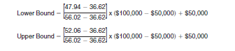
The confidence interval is $79,175 to $89,794.
6. The estimated standard error of the median is

1. The housing unit observed sampling rate in City C is 14.3. Suppose that the corresponding design factor in Table C for the housing characteristic "Value" is 1.2.
2. Obtain the frequency distribution for housing values in City C. The base is the sum of the frequencies (4,227).
| Table 1. Frequency Distribution and Cumulative Totals for Housing Value | |||
|---|---|---|---|
| Housing value | Frequency | Cumulative sum | Cumulative percent |
| Less than $50,000 | 1,548 | 1,548 | 36.62 |
| $50,000 to $99,999 | 820 | 2,368 | 56.02 |
| $100,000 to $149,999 | 752 | 3,120 | 73.81 |
| $150,000 to $199,999 | 524 | 3,644 | 86.21 |
| $200,000 to $299,999 | 300 | 3,944 | 93.30 |
| $300,000 to $499,999 | 248 | 4,192 | 99.17 |
| $500,000 or more | 35 | 4,227 | 100.00 |
3. Determine the standard error of the estimate of 50 percent from the distribution:
4. Calculate a confidence interval with bounds:
p_lower =50 -2.06 = 47.94
p_upper = 50 - 2.06 = 52.06
From the given distribution, the category with the cumulative percent first exceeding 47.94 percent is $50,000 to $99,999. Therefore, A1 = $50,000. C1 is the cumulative percent of housing units with value less than $50,000. As a result, C1 = 36.62 percent.
The category with the cumulative percent that first exceeds 52.06 percent is also $50,000 to $99,999. A2 is the smallest value in the next (higher) category, resulting in A2 = $100,000. C2 is the cumulative percent of housing units with value less than $100,000. Thus, C2 = 56.02 percent.
5. Given the values obtained in earlier steps, calculate the Lower and Upper Bounds of the confidence interval about the median:
The confidence interval is $79,175 to $89,794.
6. The estimated standard error of the median is
This example shows the steps for calculating the standard error for the average commuting time in City D. The frequency distribution is given in Table 2.
1. Cumulating the frequencies over the 12 categories for those who commuted to work (i.e., Did not work at home) yields the population count (base) of 776,619 workers age 16 years and over.
2. Find the midpoint mj for each of the 12 categories. Multiply each category's proportion pj by the square of the midpoint and sum this product over all categories. For example, the midpoint of category 1 "Less than 5 minutes" is

while the midpoint of the 12th category "90 or more minutes" is
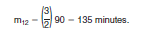
The proportion of units in the first category, p1, is

Necessary products for the standard error calculation are given in Table 3 along with totals.
3. To estimate the mean commuting time for people in City D, multiply each category's proportion by its midpoint and sum over all categories in the universe. Table 3 shows an estimated mean travel time to work, x , of 26 minutes.
4. Calculate the estimated population variance.
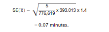
5. In City D, the person observed sampling rate is 13.1 percent. Suppose the design factor for "Travel time to work" in City D, given in the "Less than 15 percent" percent-in-sample column of Table C, is 1.4. Use this information and the results from steps 1 through 4 to calculate an estimated standard error for the mean as:
| Table 2. Frequency Distribution for Travel Time to Work | |
|---|---|
| Travel time to work | Frequency |
| Did not work at home: | 776,619 |
| Less than 5 minutes | 14,602 |
| 5 to 9 minutes | 69,066 |
| 10 to 14 minutes | 107,161 |
| 15 to 19 minutes | 138,187 |
| 20 to 24 minutes | 139,726 |
| 25 to 29 minutes | 52,879 |
| 30 to 34 minutes | 120,636 |
| 35 to 39 minutes | 19,751 |
| 40 to 44 minutes | 25,791 |
| 45 to 59 minutes | 50,322 |
| 60 to 89 minutes | 29,178 |
| 90 or more minutes | 9,320 |
| Worked at home | 19,986 |
1. Cumulating the frequencies over the 12 categories for those who commuted to work (i.e., Did not work at home) yields the population count (base) of 776,619 workers age 16 years and over.
2. Find the midpoint mj for each of the 12 categories. Multiply each category's proportion pj by the square of the midpoint and sum this product over all categories. For example, the midpoint of category 1 "Less than 5 minutes" is
while the midpoint of the 12th category "90 or more minutes" is
The proportion of units in the first category, p1, is
Necessary products for the standard error calculation are given in Table 3 along with totals.
| Table 3.Calculations for Travel Time to Work | ||||
|---|---|---|---|---|
| Travel time to work | pj | mj | pjmj 2 | pjmj |
| Did not work at home: | ||||
| Less than 5 minutes | 0.019 | 2.5 | 0.119 | 0.048 |
| 5 to 9 minutes | 0.089 | 7 | 4.361 | 0.623 |
| 10 to 14 minutes | 0.138 | 12 | 19.872 | 1.656 |
| 15 to 19 minutes | 0.178 | 17 | 51.442 | 3.026 |
| 20 to 24 minutes | 0.180 | 22 | 87.120 | 3.960 |
| 25 to 29 minutes | 0.068 | 27 | 49.572 | 1.836 |
| 30 to 34 minutes | 0.155 | 32 | 158.720 | 4.960 |
| 35 to 39 minutes | 0.025 | 37 | 34.225 | 0.925 |
| 40 to 44 minutes | 0.033 | 42 | 58.212 | 1.386 |
| 45 to 59 minutes | 0.065 | 52 | 175.760 | 3.380 |
| 60 to 89 minutes | 0.038 | 74.5 | 210.910 | 2.831 |
| 90 or more minutes | 0.012 | 135 | 218.700 | 1.620 |
| Total | 1069.013 | 26.251 | ||
3. To estimate the mean commuting time for people in City D, multiply each category's proportion by its midpoint and sum over all categories in the universe. Table 3 shows an estimated mean travel time to work, x , of 26 minutes.
4. Calculate the estimated population variance.
5. In City D, the person observed sampling rate is 13.1 percent. Suppose the design factor for "Travel time to work" in City D, given in the "Less than 15 percent" percent-in-sample column of Table C, is 1.4. Use this information and the results from steps 1 through 4 to calculate an estimated standard error for the mean as:
The estimates that appear in this product were obtained from an iterative ratio estimation procedure (iterative proportional fitting) resulting in the assignment of a weight to each sample person or housing unit record. For any given tabulation area, a characteristic total was estimated by summing the weights assigned to the people or housing units possessing the characteristic in the tabulation area. Estimates of family or household characteristics were based on the weight assigned to the family member designated as householder. Each sample person or housing unit record was assigned exactly one weight to be used to produce estimates of all characteristics. For example, if the weight given to a sample person or housing unit had the value 6, all characteristics of that person or housing unit would be tabulated with a weight of 6. The estimation procedure, however, did assign weights varying from person to person or housing unit to housing unit.
The estimation procedure used to assign the weights was performed in geographically defined weighting areas. Generally, weighting areas were formed of contiguous geographic units within counties. Weighting areas were required to have a minimum sample of 400 people. Also, weighting areas never crossed state or county boundaries. In small counties with a sample count below 400 people, the minimum sample size condition was relaxed to permit the entire county to become a weighting area.
The estimation procedure used to assign the weights was performed in geographically defined weighting areas. Generally, weighting areas were formed of contiguous geographic units within counties. Weighting areas were required to have a minimum sample of 400 people. Also, weighting areas never crossed state or county boundaries. In small counties with a sample count below 400 people, the minimum sample size condition was relaxed to permit the entire county to become a weighting area.
Within a weighting area, the long form sample was ratio-adjusted to equal the 100-percent totals for certain data groups. There were four stages of ratio adjustment for people. The first stage used 21 household-type groups. The second stage used three groups with the following sampling rates: 1-in-2, 1-in-4, and less than 1-in-4. The third stage used the dichotomy householders/nonhouseholders and the fourth stage used 312 aggregate age-sex-race-Hispanic origin groups. The stages were defined as follows:
NOTE: Multiple race people were included in one of the six race groups for estimation purposes only. Subsequent tabulations were based on the full set of responses to the race item. The ratio estimation procedure for people was conducted within a weighting area in four stages as follows:
| People | |
|---|---|
| Stage I: Type of Household | |
| Group | Family with own children under 18: Number of people in housing unit |
| 1 | 2 |
| 2 | 3 |
| 3 | 4 |
| 4 | 5 |
| 5 | 6-7 |
| 6 | 8 or more |
| Family without own children under 18: | |
| 7-12 | 2 through 8 or more |
| All other housing units: | |
| 13 | 1 |
| 14-19 | 2 through 8 or more |
| 20 | People in group quarters |
| 21 | Service Based Enumerations |
| Stage II: Sampling Type | |
| Group | |
| 1 | 1-in-2 |
| 2 | 1-in-4 |
| 3 | 1-in-6 or 1-in-8 |
| Stage III: Householder Status | |
| Group | |
| 1 | Householder |
| 2 | Nonhouseholder |
| Stage IV: Age/Sex/Race/Hispanic origin | |
| People of Hispanic origin: Black or African American: Male: | |
| Group | Age |
| 1 | 0-4 |
| 2 | 5-14 |
| 3 | 15-17 |
| 4 | 18-19 |
| 5 | 20-24 |
| 6 | 25-29 |
| 7 | 30-34 |
| 8 | 35-44 |
| 9 | 45-49 |
| 10 | 50-54 |
| 11 | 55-64 |
| 12 | 65-74 |
| 13 | 75+ |
| 14-26 | Female: Same age categories as 1-13 |
| 27-52 | American Indian or Alaska Native: Same gender and age categories as 1-26 |
| 53-78 | Asian: Same gender and age categories as 1-26 |
| 79-104 | Native Hawaiian or Pacific Islander: Same gender and age categories as 1-26 |
| 105-130 | White: Same gender and age categories as 1-26 |
| 131-156 | Some Other Race: Same gender and age categories as 1-26 |
| 157-312 | People not of Hispanic origin: Same race, gender, and age categories as 1-156 |
NOTE: Multiple race people were included in one of the six race groups for estimation purposes only. Subsequent tabulations were based on the full set of responses to the race item. The ratio estimation procedure for people was conducted within a weighting area in four stages as follows:
1. Assign an initial weight to each sample person record approximately equal to the inverse of the observed sampling rate for the weighting area.
2. Prior to iterative proportional fitting, combine categories in each of the four estimation stages, if necessary, to increase the reliability of the ratio estimation procedure. For each stage, any group that did not meet certain criteria for the unweighted sample count or for the ratio of the 100-percent to the initially weighted sample count was combined with another group in the same stage according to a specified collapsing pattern. There was an additional criterion concerning the number of complete count people in each race/Hispanic origin category in the second estimation stage.
3. The initial weights underwent four stages of ratio adjustment applying the grouping procedures described above. At the first stage, the ratio of the complete census count to the sum of the initial weights for each sample person was computed for each Stage I group. The initial weight assigned to each person in a group was then multiplied by the Stage I group ratio to produce an adjusted weight.
The Stage I adjusted weights were again adjusted by the ratio of the complete census count to the sum of the Stage I weights for sample people in each Stage II group.
The Stage II weights were adjusted by the ratio of the complete census count to the sum of the Stage II weights for sample people in each Stage III group.
The Stage III weights were adjusted by the ratio of the complete census count to the sum of the Stage III weights for sample people in each Stage IV group.
The four stages of ratio adjustment were repeated in the order given above until the predefined stopping criteria were met. The weights obtained from the final iteration of Stage IV were assigned to the sample person records. However, to avoid complications in rounding for tabulated data, only whole number weights were assigned. For example, if the final weight of the people in a particular group was 7.25, then 1/4 of the sample people in this group were randomly assigned a weight of 8, while the remaining 3/4 received a weight of 7.
The four stages of ratio adjustment were repeated in the order given above until the predefined stopping criteria were met. The weights obtained from the final iteration of Stage IV were assigned to the sample person records. However, to avoid complications in rounding for tabulated data, only whole number weights were assigned. For example, if the final weight of the people in a particular group was 7.25, then 1/4 of the sample people in this group were randomly assigned a weight of 8, while the remaining 3/4 received a weight of 7.
The ratio estimation procedure for housing units was essentially the same as that for people, except that vacant housing units were treated separately. The occupied housing unit ratio estimation procedure was done in three stages. The first stage for occupied housing units used 19 household type groups while the second stage used three sampling type groups. The third stage used 24 race-Hispanic origin-tenure groups. The vacant housing unit ratio estimation procedure was done in a single stage with three groups. The stages for ratio estimation for housing units were as follows:
The estimates produced by this estimation procedure realize some of the gains in sampling efficiency that would have resulted if the population had been stratified into the ratio-estimation groups before sampling and if the sampling rate had been applied independently to each group. The net effect is a reduction in both the standard error and the possible bias of most estimated characteristics to levels below what would have resulted from simply using the initial, unadjusted weight. A by-product of this estimation procedure is that the estimates from the sample will, for the most part, be consistent with the complete count figures for the population and housing unit groups used in the estimation procedure.
| Occupied Housing Units | |
|---|---|
| Stage I: Type of Household | |
| Group | Family with own children under 18: Number of people in housing unit |
| 1 | 2 |
| 2 | 3 |
| 3 | 4 |
| 4 | 5 |
| 5 | 6-7 |
| 6 | 8 or more |
| Family without own children under 18: | |
| 7-12 | 2 through 8 or more |
| All other housing units: | |
| 13 | 1 |
| 14-19 | 2 through 8 or more |
| Stage II: Sampling Type | |
| Group | |
| 1 | 1-in-2 |
| 2 | 1-in-4 |
| 3 | 1-in-6 or 1-in-8 |
| Stage III: Race and Hispanic Origin of Householder/Tenure | |
| Group | Owner: Hispanic origin: |
| 1 | Black or African American |
| 2 | American Indian or Alaska Native |
| 3 | Asian |
| 4 | Native Hawaiian or Pacific Islander |
| 5 | White |
| 6 | Some Other Race |
| 7-12 | Owner: Not of Hispanic origin: Same race categories as 1-6 |
| 13-24 | Renter: Same Hispanic origin and race categories as 1-12 |
| Vacant Housing Units | |
| Group | |
| 1 | Vacant for rent |
| 2 | Vacant for sale |
| 3 | Other vacant |
The estimates produced by this estimation procedure realize some of the gains in sampling efficiency that would have resulted if the population had been stratified into the ratio-estimation groups before sampling and if the sampling rate had been applied independently to each group. The net effect is a reduction in both the standard error and the possible bias of most estimated characteristics to levels below what would have resulted from simply using the initial, unadjusted weight. A by-product of this estimation procedure is that the estimates from the sample will, for the most part, be consistent with the complete count figures for the population and housing unit groups used in the estimation procedure.
As described earlier, Census 2000 long form data were collected on a sample basis. Cities and incorporated places were used to determine sampling rates to support estimates for these areas. As a result, each city, incorporated place, school district, and county had addresses selected in the long form sample.
To produce estimates from the long form data, weighting was performed at the weighting area level. In forming weighting areas, trade-offs between reliability, consistency of the estimates, and complexity of the implementation were considered. The decision was made to form weighting areas consisting of small geographic areas with at least 400 sample persons (or about 200 or more completed long forms) that do not cross county boundaries. No other boundary constraints were imposed. Thus, total population estimates from the long form data will agree with census counts reported in SF 1 and SF 2 for the weighting area, county, and other higher geographic areas obtained by combining either weighting areas or counties. Differences between long form estimates of characteristics in the SF 3 and their corresponding values in the SF 1 or SF 2 are particularly noticeable for small places, tracts, and block groups. Examples of these characteristics are the total number of people, the number of people reporting specific racial categories, and the number of housing units. The official values for items reported on the short form come from SF 1 and SF 2.
Because the weighting areas were formed at a smaller geographic level, any differential nonresponse to long form questionnaires by demographic groups or geographical areas included in a weighting area may introduce differences in complete counts (SF 1 and SF 2) and the SF 3 total population estimates. Also, an insufficient number of sample cases in the weighting matrix cells could lead to differences in SF 1, SF 2, and SF 3 population totals. Thus, differences between the census and SF 3 counts are typical and expected.
In 1990, separate tabulations were not prepared for small areas below a certain size. In contrast, Census 2000 tabulations are being prepared for all areas to maximize data availability. This approach may lead to a greater number of anomalous results than what may have been observed with tabulations released from the 1990 census. A similar phenomenon occurred in the 1990 census when weighting areas respected city and place boundaries. Census counts differed from the long form data estimates in small places. As expected, these differences were sometimes large.
The SF 1 tables provide the official census count of the number of people in an area. The SF 3 tables provide estimates of the proportion of people with specific characteristics, such as occupation, disability, or educational attainment. The total number of people in the SF 3 table is provided for use as the denominator, or base, for these proportions. Estimates in the SF 3 tables give the best estimates of the proportion of people with a particular characteristic, but the census count is the official count of how many people are in the area.
The SF 1 gives exact numbers even for very small groups and areas; whereas, SF 3 gives estimates for small groups and areas, such as tracts and small places, that are less exact. The goal of SF 3 is to identify large differences among areas or large changes over time. Estimates for small areas and small population groups often exhibit large changes from one census to the next, so having the capability to measure them is worthwhile.
In any large-scale statistical operation, such as Census 2000, human and processing errors occur. These errors are commonly referred to as nonsampling errors. Such errors include: not enumerating every household or every person in the population, failing to obtain all required information from the respondents, obtaining incorrect or inconsistent information, and recording information incorrectly. In addition, errors can occur during the field review of the enumerators work, during clerical handling of the census questionnaires, or during the electronic processing of the questionnaires.
While it is impossible to completely eliminate nonsampling error from an operation as large and complex as the decennial census, the Census Bureau attempts to control the sources of such error during the data collection and processing operations. The primary sources of nonsampling error and the programs instituted to control this error in Census 2000 are described below. The success of these programs, however, was contingent upon how well the instructions actually were carried out during the census. As part of the Census 2000 evaluation program, both the effects of these programs and the amount of error remaining after their application will be evaluated.
While it is impossible to completely eliminate nonsampling error from an operation as large and complex as the decennial census, the Census Bureau attempts to control the sources of such error during the data collection and processing operations. The primary sources of nonsampling error and the programs instituted to control this error in Census 2000 are described below. The success of these programs, however, was contingent upon how well the instructions actually were carried out during the census. As part of the Census 2000 evaluation program, both the effects of these programs and the amount of error remaining after their application will be evaluated.
Nonresponse to particular questions on the census questionnaire or the failure to obtain any information for a housing unit allows for the introduction of bias into the data because the characteristics of the nonrespondents have not been observed and may differ from those reported by respondents. As a result, any imputation procedure using respondent data may not completely reflect these differences either at the elemental level (individual person or housing unit) or on average. As part of the data processing, people and/or housing units for which sample data were not collected may have their data imputed to ensure a sufficient number of sample people/housing units in a given area. As a result, the imputation rates for some small geographic areas, such as tracts, are very high. The Census Bureau cautions data users about the impact the higher imputation rates may have on the sample characteristics. Some protection against the introduction of large biases is afforded by minimizing nonresponse. Characteristics for the nonresponses were imputed by using reported data for a person or housing unit with similar characteristics.
The person answering the mail questionnaire for a household or responding to the questions posed by an enumerator could serve as a source of error, although the question wording was extensively tested in several experimental studies prior to the census. The mail respondent may overlook or misunderstand a question, or answer a question in a way that cannot be interpreted correctly by the data capture system. Also, the enumerator may: misinterpret or otherwise incorrectly record information given by a respondent, fail to collect some of the information for a person or household, or collect data for households that were not designated as part of the sample. Enumerators were monitored carefully to minimize these types of field enumeration problems. Field staff was prepared for their tasks by using standardized training packages that included hands-on experience with census materials. A sample of the households interviewed by each enumerator was reinterviewed to control for the possibility of fabricated data being submitted by enumerators.
The many phases involved in processing the census data represent potential sources for the introduction of nonsampling error. The processing of the census questionnaires completed by enumerators included field review by the crew leader, check-in, and transmittal of completed questionnaires. No field reviews were done on the mail return questionnaires. Error may also be introduced by the misinterpretation of data by the data capture system, or the failure to capture all the information that the respondents or enumerators provided on the forms. Write-in entries go through coding operations, which may also be a source of processing error in the data. Many of the various field, coding, and computer operations undergo a number of quality control checks to help ensure their accurate application.
A number of techniques were implemented during the census planning and development stages to reduce various types of nonsampling errors. Quality assurance methods were used throughout the data collection and processing phases of the census to improve the quality of the data. In addition, the Census Bureau implemented a reinterview program to minimize errors in the data-collection phase for enumerator-filled questionnaires.
Several initiatives were implemented during Census 2000 to minimize the undercoverage of population and housing units and to reduce costs. These programs were developed based on experience from the 1990 decennial census and results from the Census 2000 testing cycle. They include:
Several initiatives were implemented during Census 2000 to minimize the undercoverage of population and housing units and to reduce costs. These programs were developed based on experience from the 1990 decennial census and results from the Census 2000 testing cycle. They include:
- Be Counted questionnaires - unaddressed forms requesting all short form data and a few additional items - were available in public locations for people who believed they were not otherwise counted.
- An introductory letter was sent to all Mailout/Mailback addresses and many addresses in Update/Leave areas prior to the mailing of the census form. A reminder postcard was also sent to these addresses.
- Forms in Spanish and other languages were mailed to those who requested them by returning the introductory letter.
- A well-publicized, toll-free telephone number was available to answer questions about the census forms. Responses from people in households who received a short form could be taken over the telephone.
- Under the Local Update of Census Addresses (LUCA) program, local officials had the opportunity to address specific concerns about the accuracy and completeness of the Master Address File before mailings began.
There were multiple modes of response for Census 2000. Because there were various ways people could initiate their enumeration in the census, and the fact that some people would be enumerated during field followup, it was very likely that some people could be enumerated more than once. A special computer process was implemented to control this type of nonsampling error by resolving situations where more than one form was received from a particular housing unit, as designated by its identification (ID). The process consisted of several steps. IDs that had more than one viable return were analyzed. Within each of these IDs, the person records on each return were compared with person records on the other return(s). People included on two or more different returns were marked as such, and only one of the person records was used in the creation of the household roster.
The objective of the processing operation was to produce a set of data that describes the population as accurately and clearly as possible. In a major change from past practice, the information on Census 2000 questionnaires generally was not edited for consistency, completeness, or acceptability during field data collection or data capture operations. Census crew leaders and local office clerks reviewed enumerator-filled questionnaires for adherence to specified procedures. Mail return questionnaires were not subjected to clerical review and households were not contacted, as in previous censuses, to collect data that were missing from census returns.
Most census questionnaires received by mail from respondents as well as those filled by enumerators were processed through a new contractor-built image scanning system that used optical mark and character recognition to convert the responses into computer files. The optical character recognition, or OCR, process used several pattern and context checks to estimate accuracy thresholds for each write-in field. The system also used "soft edits" on most interpreted numeric write-in responses to decide whether the field values read by the machine interpretation were acceptable. If the value read had a lower than acceptable accuracy threshold or was outside the soft edit range, the image of the item was displayed to a keyer who then entered the response.
To control the possible creation of erroneous people from questionnaires containing stray marks or completed incorrectly, the data capture system included an edit for the number of people indicated on each mail return and enumerator-filled questionnaire. If the edit failed, the questionnaire image was reviewed at a workstation by an operator. The operator identified erroneous person records and corrected OCR interpretation errors in the population count field.
At Census Bureau headquarters, the mail response data records were subjected to a computer edit that identified households exhibiting a possible coverage problem and those with more than six household members - the maximum number of people who could be enumerated on a mail questionnaire. Attempts were made to contact these households on the telephone to correct the count inconsistency and to collect census data for those people for whom there was no room on the questionnaire.
Incomplete or inconsistent information on the questionnaire data records was assigned acceptable values using imputation procedures during the final automated edit of the collected data. As in previous censuses, the general procedure for changing unacceptable entries was to assign an entry for a person that was consistent with entries for people with similar characteristics. Assigning acceptable codes in place of blanks or unacceptable entries enhances the usefulness of the data.
Another way in which corrections were made during the computer editing process was substitution. Substitution assigned a full set of characteristics for people in a household. If there was an indication that a household was occupied by a specified number of people but the questionnaire contained no information for people within the household, or the occupants were not listed on the questionnaire, the Census Bureau selected a previously accepted household of the same size and substituted its full set of characteristics for this household.
1For estimated totals larger than 10,000,000, the standard error is somewhat larger than the table values. Use the formula given below to calculate the standard error.
2The total count of people, housing units, households, or families in the area if the estimated total is a person, housing unit, household, or family characteristic, respectively.
The 5 in the above equation is based on a 1-in-6 sample and is derived from the inverse of the sampling rate minus one, i.e., 5 = 6 1 .
1For a percentage and/or base of percentage not shown in the table, use the formula given below to calculate the standard error. Use this table only for proportions; that is, where the numerator is a subset of the denominator.
The 5 in the above equation is based on a 1-in-6 sample and is derived from the inverse of the sampling rate minus one, i.e., 5 = 6 1 .
Most census questionnaires received by mail from respondents as well as those filled by enumerators were processed through a new contractor-built image scanning system that used optical mark and character recognition to convert the responses into computer files. The optical character recognition, or OCR, process used several pattern and context checks to estimate accuracy thresholds for each write-in field. The system also used "soft edits" on most interpreted numeric write-in responses to decide whether the field values read by the machine interpretation were acceptable. If the value read had a lower than acceptable accuracy threshold or was outside the soft edit range, the image of the item was displayed to a keyer who then entered the response.
To control the possible creation of erroneous people from questionnaires containing stray marks or completed incorrectly, the data capture system included an edit for the number of people indicated on each mail return and enumerator-filled questionnaire. If the edit failed, the questionnaire image was reviewed at a workstation by an operator. The operator identified erroneous person records and corrected OCR interpretation errors in the population count field.
At Census Bureau headquarters, the mail response data records were subjected to a computer edit that identified households exhibiting a possible coverage problem and those with more than six household members - the maximum number of people who could be enumerated on a mail questionnaire. Attempts were made to contact these households on the telephone to correct the count inconsistency and to collect census data for those people for whom there was no room on the questionnaire.
Incomplete or inconsistent information on the questionnaire data records was assigned acceptable values using imputation procedures during the final automated edit of the collected data. As in previous censuses, the general procedure for changing unacceptable entries was to assign an entry for a person that was consistent with entries for people with similar characteristics. Assigning acceptable codes in place of blanks or unacceptable entries enhances the usefulness of the data.
Another way in which corrections were made during the computer editing process was substitution. Substitution assigned a full set of characteristics for people in a household. If there was an indication that a household was occupied by a specified number of people but the questionnaire contained no information for people within the household, or the occupants were not listed on the questionnaire, the Census Bureau selected a previously accepted household of the same size and substituted its full set of characteristics for this household.
| Table A. Unadjusted Standard Error for Estimated Totals [Based on a 1-in-6 simple random sample] | |||||||||||||||
|---|---|---|---|---|---|---|---|---|---|---|---|---|---|---|---|
| Estimated total1 | Size of publication area2 | ||||||||||||||
| 500 | 1,000 | 2,500 | 5,000 | 10,000 | 25,000 | 50,000 | 100,000 | 250,000 | 500,000 | 1,000,000 | 5,000,000 | 10,000,000 | 25,000,000 | ||
| 50 | 15 | 15 | 16 | 16 | 16 | 16 | 16 | 16 | 16 | 16 | 16 | 16 | 16 | 16 | |
| 100 | 20 | 21 | 22 | 22 | 22 | 22 | 22 | 22 | 22 | 22 | 22 | 22 | 22 | 22 | |
| 250 | 25 | 31 | 34 | 34 | 35 | 35 | 35 | 35 | 35 | 35 | 35 | 35 | 35 | 35 | |
| 500 | - | 35 | 45 | 47 | 49 | 49 | 50 | 50 | 50 | 50 | 50 | 50 | 50 | 50 | |
| 1,000 | - | - | 55 | 63 | 67 | 69 | 70 | 70 | 71 | 71 | 71 | 71 | 71 | 71 | |
| 2,500 | - | - | - | 79 | 97 | 106 | 109 | 110 | 111 | 112 | 112 | 112 | 112 | 112 | |
| 5,000 | - | - | - | - | 112 | 141 | 150 | 154 | 157 | 157 | 158 | 158 | 158 | 158 | |
| 10,000 | - | - | - | - | - | 173 | 200 | 212 | 219 | 221 | 222 | 223 | 223 | 224 | |
| 15,000 | - | - | - | - | - | 173 | 229 | 252 | 266 | 270 | 272 | 273 | 274 | 274 | |
| 25,000 | - | - | - | - | - | - | 250 | 306 | 335 | 345 | 349 | 353 | 353 | 353 | |
| 75,000 | - | - | - | - | - | - | - | 306 | 512 | 565 | 589 | 608 | 610 | 611 | |
| 100,000 | - | - | - | - | - | - | - | - | 548 | 632 | 671 | 700 | 704 | 706 | |
| 250,000 | - | - | - | - | - | - | - | - | - | 791 | 968 | 1090 | 1104 | 1112 | |
| 500,000 | - | - | - | - | - | - | - | - | - | - | 1118 | 1500 | 1541 | 1565 | |
| 1,000,000 | - | - | - | - | - | -- | - | - | - | - | - | 2000 | 2121 | 2191 | |
| 5,000,000 | - | - | - | - | - | - | - | - | - | - | - | - | 3536 | 4472 | |
| 10,000,000 | - | - | - | - | - | - | - | - | - | - | - | - | - | 5477 | |
Footnotes:
1For estimated totals larger than 10,000,000, the standard error is somewhat larger than the table values. Use the formula given below to calculate the standard error.
2The total count of people, housing units, households, or families in the area if the estimated total is a person, housing unit, household, or family characteristic, respectively.
The 5 in the above equation is based on a 1-in-6 sample and is derived from the inverse of the sampling rate minus one, i.e., 5 = 6 1 .
| Table B. Unadjusted Standard Error in Percentage Points for Estimated Percentages [Based on a 1-in-6 simple random sample] | ||||||||||||||
|---|---|---|---|---|---|---|---|---|---|---|---|---|---|---|
| Estimated percentage | Base of estimated percentage1 | |||||||||||||
| 500 | 750 | 1,000 | 1,500 | 2,500 | 5,000 | 7,500 | 10,000 | 25,000 | 50,000 | 100,000 | 250,000 | 500,000 | ||
| 2 or 98 | 14 | 11 | 10 | 08 | 06 | 04 | 04 | 03 | 02 | 01 | 01 | 01 | 00 | |
| 5 or 95 | 22 | 18 | 15 | 13 | 10 | 07 | 06 | 05 | 03 | 02 | 02 | 01 | 01 | |
| 10 or 90 | 30 | 24 | 21 | 17 | 13 | 09 | 08 | 07 | 04 | 03 | 02 | 01 | 01 | |
| 15 or 85 | 36 | 29 | 25 | 21 | 16 | 11 | 09 | 08 | 05 | 04 | 03 | 02 | 01 | |
| 20 or 80 | 40 | 33 | 28 | 23 | 18 | 13 | 10 | 09 | 06 | 04 | 03 | 02 | 01 | |
| 25 or 75 | 43 | 35 | 31 | 25 | 19 | 14 | 11 | 10 | 06 | 04 | 03 | 02 | 01 | |
| 30 or 70 | 46 | 37 | 32 | 26 | 20 | 14 | 12 | 10 | 06 | 05 | 03 | 02 | 01 | |
| 35 or 65 | 48 | 39 | 34 | 28 | 21 | 15 | 12 | 11 | 07 | 05 | 03 | 02 | 02 | |
| 50 | 50 | 41 | 35 | 29 | 22 | 16 | 13 | 11 | 07 | 05 | 04 | 02 | 02 | |
Footnotes:
1For a percentage and/or base of percentage not shown in the table, use the formula given below to calculate the standard error. Use this table only for proportions; that is, where the numerator is a subset of the denominator.
The 5 in the above equation is based on a 1-in-6 sample and is derived from the inverse of the sampling rate minus one, i.e., 5 = 6 1 .

