


| Documentation: | ACS 2019 (5-Year Estimates) |
you are here:
choose a survey
survey
document
chapter
Publisher: U.S. Census Bureau
Survey: ACS 2019 (5-Year Estimates)
| Document: | 2019 ACS 1-year and 2015-2019 ACS 5-year Data Releases: Technical Documentation |
| citation: | Social Explorer; U.S. Census Bureau; 2019 ACS 1-year and 2015-2019 ACS 5-year Data Releases : Technical Documentation. |
Chapter Contents
This document describes the accuracy of the 2019 American Community Survey (ACS) 1-year estimates. The data contained in these data products are based on the sample interviewed from January 1, 2019 through December 31, 2019.
The ACS sample is selected from all counties and county-equivalents in the United States. In 2006, the ACS began collecting data from sampled persons in group quarters (GQs) - for example, military barracks, college dormitories, nursing homes, and correctional facilities. Persons in sample in (GQs) and persons in sample in housing units (HUs) are included in all 2019 ACS estimates that are based on the total population. All ACS population estimates from years prior to 2006 include only persons in housing units.
The ACS, like any other sample survey, is subject to error. The purpose of this document is to provide data users with a basic understanding of the ACS sample design, estimation methodology, and the accuracy of the ACS data. The ACS is sponsored by the U.S. Census Bureau, and is part of the Decennial Census Program.
For additional information on the design and methodology of the ACS, including data collection and processing, visit: https://www.census.gov/programs-surveys/acs/methodology.html.
To access other accuracy of the data documents, including the 2019 PRCS Accuracy of the Data document and the 2015-2019 ACS Accuracy of the Data document1, visit: https://www.census.gov/programs-surveys/acs/technical-documentation/code-lists.html.
Footnotes:
1 The 2015-2019 Accuracy of the Data document will be available after the release of the 5-year products in December 2019.
The ACS employs three modes of data collection:
With the exception of addresses in Remote Alaska, the general timing of data collection is:
Month 1: Addresses in sample that are determined to be mailable are sent an initial mailing package - this package contains information for completing the ACS questionnaire on the internet (on-line). If a sample address has not responded online within approximately two weeks of the initial mailing, then a second mailing package with a paper questionnaire is sent. Sampled addresses then have the option of which mode to use to complete the interview.
Month 2: All mail non-responding addresses with an available phone number are sent to CATI.
Month 3: A sample of mail non-responses without a phone number, CATI non-responses, and unmailable addresses are selected and sent to CAPI.
Note that mail responses are accepted during all three months of data collection.
All remote Alaska addresses in sample are sent to CAPI and assigned to one of two data collection periods: January-April or September-December.3 Up to four months is allowed to complete the assigned interviews. As we do not mail to any remote Alaska addresses, this is the only data collection mode available.
Footnotes:
2 Note that all CATI operations ended at the end of September, 2017
3 Prior to the 2011 sample year, all remote Alaska sample cases were subsampled for CAPI at a rate of 2-in-3.
- Internet
- Mailout/Mailback
- Computer Assisted Telephone Interview (CATI)2
- Computer Assisted Personal Interview (CAPI)
With the exception of addresses in Remote Alaska, the general timing of data collection is:
Month 1: Addresses in sample that are determined to be mailable are sent an initial mailing package - this package contains information for completing the ACS questionnaire on the internet (on-line). If a sample address has not responded online within approximately two weeks of the initial mailing, then a second mailing package with a paper questionnaire is sent. Sampled addresses then have the option of which mode to use to complete the interview.
Month 2: All mail non-responding addresses with an available phone number are sent to CATI.
Month 3: A sample of mail non-responses without a phone number, CATI non-responses, and unmailable addresses are selected and sent to CAPI.
Note that mail responses are accepted during all three months of data collection.
All remote Alaska addresses in sample are sent to CAPI and assigned to one of two data collection periods: January-April or September-December.3 Up to four months is allowed to complete the assigned interviews. As we do not mail to any remote Alaska addresses, this is the only data collection mode available.
Footnotes:
2 Note that all CATI operations ended at the end of September, 2017
3 Prior to the 2011 sample year, all remote Alaska sample cases were subsampled for CAPI at a rate of 2-in-3.
Group Quarters data collection spans six weeks, except in Remote Alaska and for Federal prisons, where the data collection time period is four months. As is done for housing unit (HU) addresses, Group Quarters in Remote Alaska are assigned to one of two data collection periods, January-April, or September-December and up to four months is allowed to complete the interviews. Similarly, all Federal prisons are assigned to September with a four month data collection window.
Field representatives have several options available to them for data collection. These include completing the questionnaire while speaking to the resident in person or over the telephone, conducting a personal interview with a proxy, such as a relative or guardian, or leaving paper questionnaires for residents to complete for themselves and then pick them up later. This last option is used for data collection in Federal prisons.
Field representatives have several options available to them for data collection. These include completing the questionnaire while speaking to the resident in person or over the telephone, conducting a personal interview with a proxy, such as a relative or guardian, or leaving paper questionnaires for residents to complete for themselves and then pick them up later. This last option is used for data collection in Federal prisons.
The universe for the ACS consists of all valid, residential housing unit addresses in all county and county equivalents in the 50 states, including the District of Columbia that are eligible for data collection. Beginning with the 2019 sample, we restricted the universe of eligible addresses further to exclude a small proportion of addresses that do not meet a set of minimum address criteria. The Master Address File (MAF) is a database maintained by the Census Bureau containing a listing of residential, group quarters, and commercial addresses in the U.S. and Puerto Rico. The MAF is normally updated twice each year with the Delivery Sequence Files (DSF) provided by the U.S. Postal Service. The DSF covers only the U.S. These files identify mail drop points and provide the best available source of changes and updates to the housing unit inventory. The MAF is also updated with the results from various Census Bureau field operations, including the ACS.
Due to operational difficulties associated with data collection, the ACS excludes certain types of GQs from the sampling universe and data collection operations. The weighting and estimation accounts for this segment of the population as they are included in the population controls. The following GQ types are those that are removed from the GQ universe:
- Soup kitchens
- Domestic violence shelters
- Regularly scheduled mobile food vans
- Targeted non-sheltered outdoor locations
- Maritime/merchant vessels
- Living quarters for victims of natural disasters
- Dangerous encampments
The ACS employs a two-phase, two-stage sample design. The first-phase sample consists of two separate address samples: Period 1 and Period 2. These samples are chosen at different points in time. Both samples are selected in two stages of sampling, a first-stage and a secondstage. Subsequent to second-stage sampling, the majority of sample addresses are randomly assigned to one of the twelve months of the sample year (the exception is for addresses in remote Alaska, which are assigned to either January or September). The second-phase of sampling occurs when the CAPI sample is selected.
The Period 1 sample is selected during September and October of the year prior to the sample year (the 2019 Period 1 sample was selected in September and October of 2017). Approximately half of a year's sample is selected at this time. Sample addresses that are not in remote Alaska are randomly assigned to one of the first six months of the sample year; sample addresses in remote Alaska are assigned to January.
Period 2 sampling occurs in January and February of the sample year (the 2019 Period 2 sample was selected during January and February of 2019). This sample accounts for the remaining half of the overall first-phase sample. Period 2 sample addresses that are not in remote Alaska are randomly assigned to one of the last six months of the sample year; Period 2 sample addresses in remote Alaska are assigned to September.4
A sub-sample of non-responding addresses and of any addresses deemed unmailable is selected for the CAPI data collection mode.5
The following steps are used to select the first-phase and second-phase samples in both periods.
Footnotes:
4 Remote Alaska assignments are made so that the sample addresses are approximately evenly distributed between the two data collection periods.
5 Beginning with the August, 2011 CAPI sample all non-mailable and non-responding addresses in the following areas are now sent to CAPI: all Hawaiian Homelands, all Alaska Native Village Statistical areas, American Indian areas with an estimated proportion of American Indian population ≥ 10%
First stage sampling defines the universe for the second stage of sampling through three steps. First, all addresses that were in a first-phase sample within the past four years are excluded from eligibility. This ensures that no address is in sample more than once in
any five-year period. The second step is to select a 20 percent systematic sample of "new" units, i.e. those units that have never appeared on a previous MAF extract within each county. Each new address is systematically assigned either to the current year or to
one of four back-samples. This procedure maintains five equal partitions (samples) of the universe. The third step is to randomly assign all eligible addresses to a period. 6
Footnotes:
6Most of the period assignments are made during Period 1 sampling. The only assignments in Period 2 sampling are made for addresses that were not part of the process in Period 1, e.g., new addresses.
Footnotes:
6Most of the period assignments are made during Period 1 sampling. The only assignments in Period 2 sampling are made for addresses that were not part of the process in Period 1, e.g., new addresses.
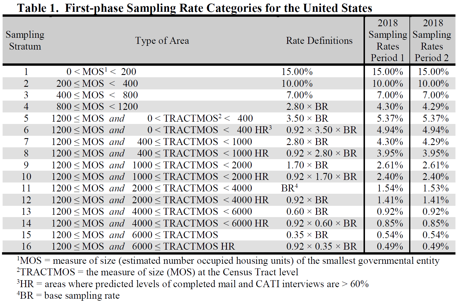
Second-stage sampling uses 16 sampling strata in the U.S.7 The stratum-level rates used
in second-stage sampling account for the first-stage selection probabilities. These rates
are applied at a block level to addresses in the U.S. by calculating a measure of size for
each of the following geographic entities:
For American Indian, Tribal Subdivisions, and Alaska Native Village Statistical Areas, the measure of size is the estimated number of occupied HUs multiplied by the proportion of people reporting American Indian or Alaska Native (alone or in combination) in the most recent Census. For Hawaiian Homelands, the measure of size is the estimated number of occupied HUs multiplied by the proportion of people reporting Native Hawaiian (alone or in combination) in the most recent Census.
Each block is then assigned the smallest positive, non-zero measure of size from the set of all entities of which it is a part. The 2019 second-stage sampling strata and the overall first-phase sampling rates by Period are shown in Table 1 below.
Footnotes:
7Beginning with the 2011 sample the ACS implemented a change to the stratification, increasing the number of sampling strata and changing how the sampling rates are defined. Prior to 2011 there were seven strata; there are now 16 sampling strata. Table 1 gives a summary of these strata and the rates.
8These are the states where MCDs are active, functioning governmental units.
- Counties Places School Districts (elementary, secondary, and unified) American Indian Areas Tribal Subdivisions Alaska Native Village Statistical Areas Hawaiian Homelands Minor Civil Divisions - in Connecticut, Maine, Massachusetts, Michigan, Minnesota, New Hampshire, New Jersey, New York, Pennsylvania, Rhode Island, Vermont, and Wisconsin8 Census Designated Places - in Hawaii only
For American Indian, Tribal Subdivisions, and Alaska Native Village Statistical Areas, the measure of size is the estimated number of occupied HUs multiplied by the proportion of people reporting American Indian or Alaska Native (alone or in combination) in the most recent Census. For Hawaiian Homelands, the measure of size is the estimated number of occupied HUs multiplied by the proportion of people reporting Native Hawaiian (alone or in combination) in the most recent Census.
Each block is then assigned the smallest positive, non-zero measure of size from the set of all entities of which it is a part. The 2019 second-stage sampling strata and the overall first-phase sampling rates by Period are shown in Table 1 below.
Footnotes:
7Beginning with the 2011 sample the ACS implemented a change to the stratification, increasing the number of sampling strata and changing how the sampling rates are defined. Prior to 2011 there were seven strata; there are now 16 sampling strata. Table 1 gives a summary of these strata and the rates.
8These are the states where MCDs are active, functioning governmental units.
The overall first-phase sampling rates are calculated using the distribution of ACS valid, eligible addresses by second-stage sampling stratum in such a way as to yield an overall target sample size for the year of 3,540,000 (1,770,000 for each period) in the U.S. The first-phase rates are adjusted for the first-stage sample to yield the second-stage selection probabilities.
After each block is assigned to a second-stage sampling stratum in each period, a systematic sample of addresses is selected from the second-stage universe (first-stage sample) within each county and county equivalent.
After the second stage of sampling, addresses selected during Period 1 sampling that are not in remote Alaska are randomly assigned to one of the first six months of the sample year. Sample addresses selected during Period 2 sampling that are not in remote Alaska are randomly assigned to a month from July through December, inclusive. Sample addresses in remote Alaska are assigned to the January or September panel in Period 1 and Period 2 sampling, respectively.
The addresses from which CAPI sub-samples are selected can be divided into two groups. One group includes addresses that are not eligible for any other data collection operation - these consist of unmailable addresses and those in remote Alaska areas. The second group includes addresses that are eligible for the other data collection operations but for which no response was obtained prior to CAPI sub-sampling - these consist of mailable addresses not in a remote Alaska area.
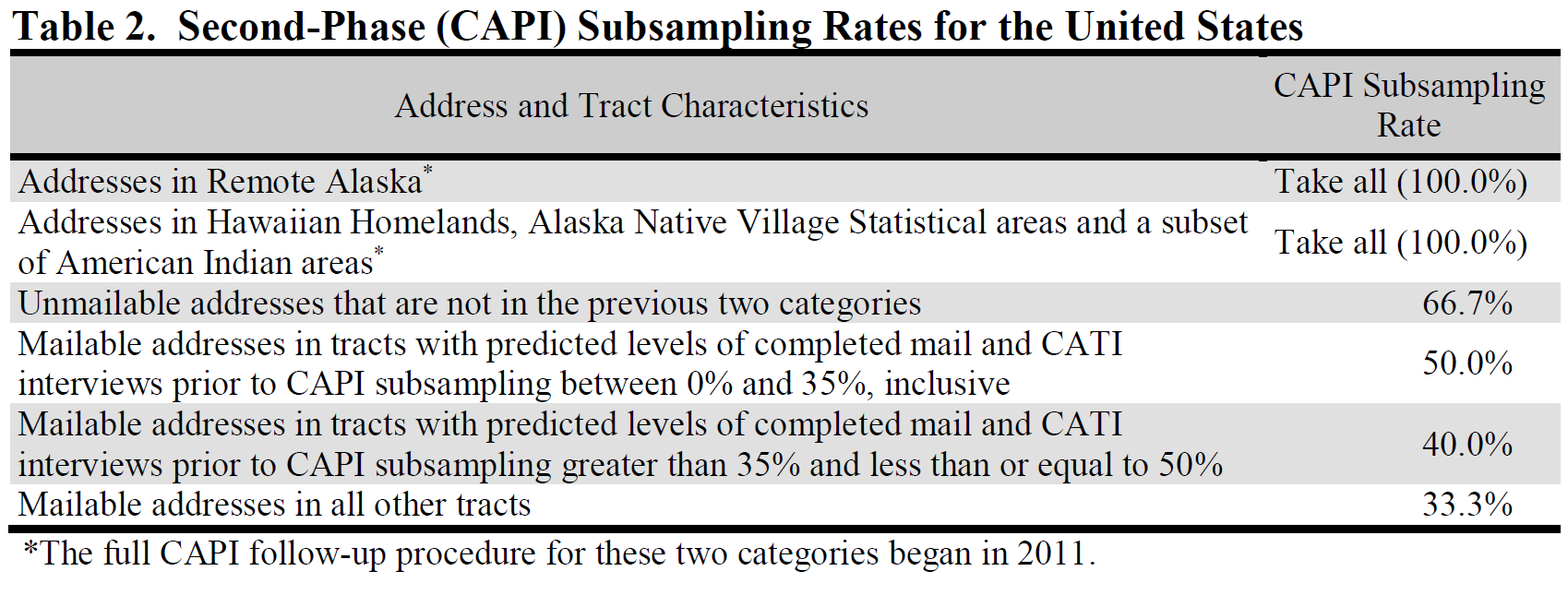
All sample addresses in remote Alaska are sent to the CAPI data collection operation. Most unmailable addresses are selected for CAPI at a rate of 2-in-3 - the exception is when they are in a Hawaiian Homeland area (HH), Alaska Native Village Statistical area (ANVSA), or pre-determined American Indian areas (AI), where all are selected for CAPI.
With one exception, mailable addresses from which a response was not obtained by the time of the CAPI operation are sampled at rates of 1-in-2, 2-in-5, and 1-in-3 - these rates are set at the tract level. The exception is for addresses in HH, ANVSA, and AI areas, where all are selected for CAPI. Table 2 shows the CAPI sub-sampling rates that are associated with each group of addresses.
The 2019 group quarters (GQ) sampling frame was divided into two strata: a small GQ stratum and a large GQ stratum. Small GQs are defined to have expected populations of fifteen or fewer residents, while large GQs have expected populations of more than fifteen residents.
Samples were selected in two phases within each stratum. In general, GQs were selected in the first phase and then persons/residents were selected in the second phase. Both phases differ between the two strata. Each sampled GQ was randomly assigned to one or more months in 2019 - it was in these months that their person samples were selected.
Samples were selected in two phases within each stratum. In general, GQs were selected in the first phase and then persons/residents were selected in the second phase. Both phases differ between the two strata. Each sampled GQ was randomly assigned to one or more months in 2019 - it was in these months that their person samples were selected.
There were two stages of selecting small GQs for sample.
- First stage
The small GQ universe is divided into five groups that are approximately equal in size. All new small GQs are systematically assigned to one of these five groups on a yearly basis, with about the same probability (20 percent) of being assigned to any given group. Each group represents a second-stage sampling frame, from which GQs are selected once every five years. The 2019 secondstage sampling frame was used in 2013 as well, and is currently to be used in 2023, 2028, etc. - Second stage
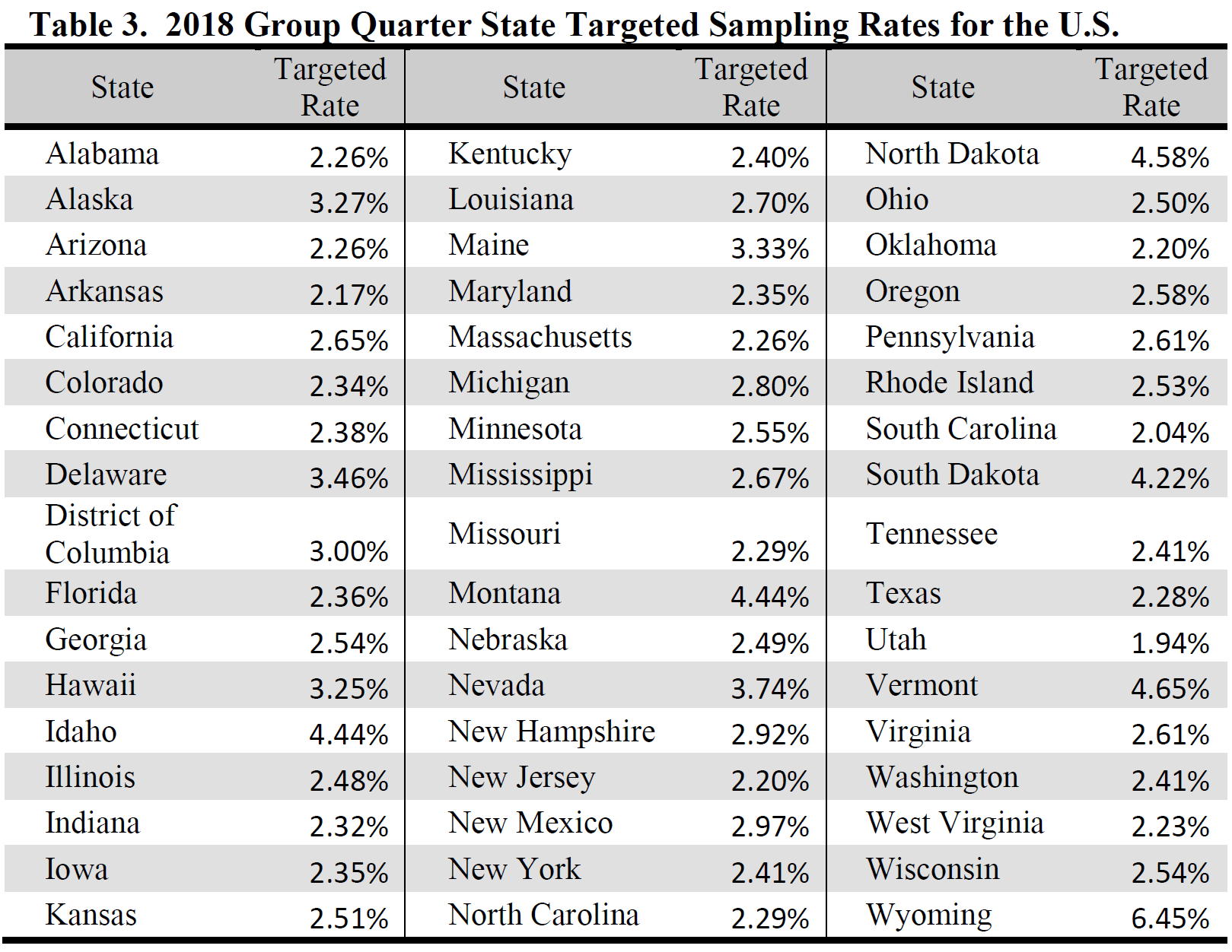
GQs were systematically selected from the 2019 second-stage sampling frame. Each GQ had the same second-stage probability of being selected within a given state, where the probabilities varied between states. Table 3 below shows these probabilities.
Persons were selected for sample from each GQ that was selected for sample in the first phase of sample selection. If fifteen or fewer persons were residing at a GQ at the time a field representative (interviewer) visited the GQ, then all persons were selected for
sample. Otherwise, if more than fifteen persons were residing at the GQ, then the interviewer selected a systematic sample of ten persons from the GQ's roster.
The targeted state-level sampling rates are the probabilities of selecting any given person in a GQ; it is around these probabilities that the sample design is based. These probabilities reflect both phases of sample selection, and they varied by state. The
probabilities for 2019 are shown in Table 3.
The sample was designed so that the second-phase sampling rate would be one-hundred percent for small GQs (i.e., select the entire expected population of fifteen or fewer persons for sample in every small sampled GQ). This means the probability of selecting any person in a small GQ was designed to equal the probability of selecting the small GQ itself.
The sample was designed so that the second-phase sampling rate would be one-hundred percent for small GQs (i.e., select the entire expected population of fifteen or fewer persons for sample in every small sampled GQ). This means the probability of selecting any person in a small GQ was designed to equal the probability of selecting the small GQ itself.
All large GQs are eligible to be sampled as has been the case every year since the inception of the GQ sampling in 2006. This means there was only a single stage of sampling in this phase. This stage consists of systematically assigning "hits" to GQs
independently in each state, where each hit represents ten persons to be sampled.
In general, a GQ has either Z or Z+1 hits assigned to it. The value for Z is dependent on both the GQ's expected population size and its within-state target sampling rate, shown in Table 3. When this rate is multiplied by a GQ's expected population, the result is a GQ's expected person sample size. If a GQ's expected person sample size is less than ten, then Z = 0; if it is at least ten but less than twenty, then Z = 1; if it is at least twenty but less than thirty, then Z = 2; and so on. See below for a detailed example.
If a GQ has an expected person sample size that is less than ten, then this method effectively gives the GQ a probability of selection that is proportional to its size; this probability is the expected person sample size divided by ten. If a GQ has an expected person sample size of ten or more, then it is in sample with certainty and is assigned one or more hits.
Persons were selected within each GQ to which one or more hits were assigned in the first phase of selection. There were ten persons selected at a GQ for every hit assigned to the GQ. The persons were systematically sampled from a roster of persons residing at the GQ at the time of an interviewer's visit. The exception was if there were far fewer persons residing in a GQ than expected - in these situations, the number of persons to sample at the GQ would be reduced to reflect the GQ's actual population. In cases where
fewer than ten persons resided in a GQ at the time of a visit, the interviewer would select all of the persons for sample.
As for small GQs, the targeted state-level sampling rates are the probabilities of selecting any given person in a GQ. The probabilities are shown in Table 3. Note that these rates are the same as for persons in small GQs.
As an example, suppose a GQ in a state had an expected population of 250, and the target sampling rate in the state was 2.29%, meaning any given person in a GQ in the state had about a 1-in-43⅔ chance of being selected. This rate, combined with the GQs expected population of 250, means that the expected number of persons selected for sample in this GQ would be 5.725 (2.29% x 250). Since this is less than ten, this GQ would have either 0 or 1 hits assigned to it (Z = 0). The probability of it being assigned a hit would be the GQ's expected person sample size of 5.725 divided by 10, or 57.25%.
As a second example, suppose a GQ in another state had an expected population of 1,000 and the target sampling rate in the state was 4.30%; this means any given person in a GQ in this state had about a 1-in-23.26 chance of being selected. This rate, combined with the GQ's expected population of 1,000, means that the expected number of persons selected for sample in the GQ would be 43 (4.30% x 1,000); this GQ would be assigned either four or five hits (Z = 4).
All sample GQs were assigned to one or more months (interview months) - these were the months in which interviewers would visit a GQ to select a person sample and conduct interviews. All small GQs, all large GQs that were assigned only one hit, all remote Alaska GQs, all sampled military facilities, and all sampled correctional facilities (regardless of how many hits a military or correctional facility was assigned) were assigned to a single interview month. Remote Alaska GQs were assigned to either January or September; Federal prisons were assigned to September; all of the others were randomly assigned one interview month.
All large GQs that had been assigned multiple hits, but were not in any of the categories above, had each hit randomly assigned to a different interview month. If a GQ had more than twelve hits assigned to it, then multiple hits would be assigned to one or more interview months for the GQ. For example, if a GQ had fifteen hits assigned to it, then there would be three interview months in which two hits were assigned and nine interview months in which one hit was assigned. There are two restrictions to this process. One restriction is applied to college dormitories, whose hits are randomly assigned to non-summer months only, i.e., January through April and September through December. The other restriction is applied to military ships, whose hits were randomly assigned only to the last ten months of the year, i.e., March through December.
All large GQs that had been assigned multiple hits, but were not in any of the categories above, had each hit randomly assigned to a different interview month. If a GQ had more than twelve hits assigned to it, then multiple hits would be assigned to one or more interview months for the GQ. For example, if a GQ had fifteen hits assigned to it, then there would be three interview months in which two hits were assigned and nine interview months in which one hit was assigned. There are two restrictions to this process. One restriction is applied to college dormitories, whose hits are randomly assigned to non-summer months only, i.e., January through April and September through December. The other restriction is applied to military ships, whose hits were randomly assigned only to the last ten months of the year, i.e., March through December.
Prior to 2016, all GQs were sampled at the same time for a given year. Starting in 2016, Bureau of Prison GQs (Federal prisons) started to be sampled separately from other GQs. They are sampled using the same procedure described above, and are all assigned to the September interview month as before.
Counts of sample addresses and GQ persons can be found in two locations on the US Census Bureau website. In American Fact Finder, base tables B98001 and B98002 provide sample size counts for the nation, states, and counties. Sample size counts for the nation and states are also available in the Sample Size and Data Quality Section of the ACS website, at https://www.census.gov/acs/www/methodology/sample-size-and-data-quality/.
Counts of sample addresses and GQ persons can be found in two locations on the US Census
Bureau website. On data.census.gov, base tables B98001 and B98002 provide sample size
counts for the nation, states, and counties. Sample size counts for the nation and states are also
available in the Sample Size and Data Quality Section of the ACS website, at
https://www.census.gov/acs/www/methodology/sample-size-and-data-quality
The estimates that appear in this product are obtained from a raking ratio estimation procedure that results in the assignment of two sets of weights: a weight to each sample person record and a weight to each sample housing unit record. Estimates of person characteristics are based on the person weight. Estimates of family, household, and housing unit characteristics are based on the housing unit weight. For any given tabulation area, a characteristic total is estimated by summing the weights assigned to the persons, households, families or housing units possessing the characteristic in the tabulation area. Each sample person or housing unit record is assigned exactly one weight to be used to produce estimates of all characteristics. For example, if the weight given to a sample person or housing unit has a value 40, all characteristics of that person or housing unit are tabulated with the weight of 40.
The weighting is conducted in two main operations: a group quarters person weighting operation which assigns weights to persons in group quarters, and a household person weighting operation which assigns weights both to housing units and to persons within housing units. The group quarters person weighting is conducted first and the household person weighting second. The household person weighting is dependent on the group quarters person weighting because estimates for total population, which include both group quarters and household population, are controlled to the Census Bureau's official 2019 total resident population estimates.
The weighting is conducted in two main operations: a group quarters person weighting operation which assigns weights to persons in group quarters, and a household person weighting operation which assigns weights both to housing units and to persons within housing units. The group quarters person weighting is conducted first and the household person weighting second. The household person weighting is dependent on the group quarters person weighting because estimates for total population, which include both group quarters and household population, are controlled to the Census Bureau's official 2019 total resident population estimates.
Starting with the weighting for the 2011 1-year ACS estimates, the group quarters (GQ) person weighting changed in important ways from previous years' weighting. The GQ population sample was supplemented by a large-scale whole person imputation into not-in-sample GQ facilities. For the 2019 ACS GQ data, roughly as many GQ persons were imputed as interviewed. The goal of the imputation methodology was two-fold.
The GQ sampling frame was modified to create an imputation frame from which all imputed GQs were selected from. The frame was updated with the actual populations and GQ type changes from ACS interviews, as well as any subsequent information gathered in other processes since the sampling frame was initially created. The change in populations for ACS GQ interviews was used to calculate a not-in-sample adjustment factor that was used to update the population for all GQs on the frame not selected for sample. This adjustment factor was calculated at the following level:
GQ Major Type x GQ Size Stratum
There were three size strata used for this process: GQs in sample with certainty, GQs with 16 or more persons, and GQs with less than 16 persons.
For all not-in-sample GQ facilities with an expected population of 16 or more persons (large facilities), we imputed a number of GQ persons equal to 2.5% of the expected population. For those GQ facilities with an expected population of fewer than 16 persons (small facilities), we selected a random sample of GQ facilities as needed to accomplish the two objectives given above. For those selected small GQ facilities, we imputed a number of GQ persons equal to 20% of the facility's expected population.
Interviewed GQ person records were then sampled at random to be donors for the imputed persons of the selected not-in-sample GQ facilities. An expanding search algorithm searched for donors within the same specific type of GQ facility and the same county. If that failed, the search included all GQ facilities of the same major GQ type group. If that still failed, the search expanded to a specific type within state, then a major GQ type group within state. This expanding search continued through division, region, and the entire nation until suitable donors were found.
The weighting procedure made no distinction between sampled and imputed GQ person records. The initial weights of person records in the large GQ facilities equaled the observed or expected population of the GQ facility divided by the number of person records. The initial weights of person records in small GQ facilities equaled the observed or expected population of the GQ facility divided by the number of records, multiplied by the inverse of the fraction of small GQ facilities represented in the weighting to the number on the frame of that tract by major GQ type group combination.
The population totals on the imputation frame are used to ensure that the sub-state distribution of GQ weighting preserves the distribution from the frame. This accomplished through a series of three constraints:
Lastly, the final GQ person weight was rounded to an integer. Rounding was performed so that the sum of the rounded weights were within one person of the sum of the unrounded weights for any of the groups listed below:
Major GQ Type Group
Major GQ Type Group x County
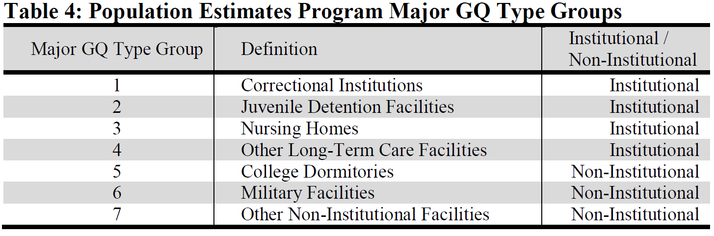
- The primary objective was to establish representation of county by major GQ type group in the tabulations for each combination that exists on the ACS GQ sample frame. The seven major GQ type groups are defined by the Population Estimates Program and are given in Table 4.
- A secondary objective was to establish representation of tract by major GQ type group for each combination that exists on the ACS GQ sample frame.
The GQ sampling frame was modified to create an imputation frame from which all imputed GQs were selected from. The frame was updated with the actual populations and GQ type changes from ACS interviews, as well as any subsequent information gathered in other processes since the sampling frame was initially created. The change in populations for ACS GQ interviews was used to calculate a not-in-sample adjustment factor that was used to update the population for all GQs on the frame not selected for sample. This adjustment factor was calculated at the following level:
GQ Major Type x GQ Size Stratum
There were three size strata used for this process: GQs in sample with certainty, GQs with 16 or more persons, and GQs with less than 16 persons.
For all not-in-sample GQ facilities with an expected population of 16 or more persons (large facilities), we imputed a number of GQ persons equal to 2.5% of the expected population. For those GQ facilities with an expected population of fewer than 16 persons (small facilities), we selected a random sample of GQ facilities as needed to accomplish the two objectives given above. For those selected small GQ facilities, we imputed a number of GQ persons equal to 20% of the facility's expected population.
Interviewed GQ person records were then sampled at random to be donors for the imputed persons of the selected not-in-sample GQ facilities. An expanding search algorithm searched for donors within the same specific type of GQ facility and the same county. If that failed, the search included all GQ facilities of the same major GQ type group. If that still failed, the search expanded to a specific type within state, then a major GQ type group within state. This expanding search continued through division, region, and the entire nation until suitable donors were found.
The weighting procedure made no distinction between sampled and imputed GQ person records. The initial weights of person records in the large GQ facilities equaled the observed or expected population of the GQ facility divided by the number of person records. The initial weights of person records in small GQ facilities equaled the observed or expected population of the GQ facility divided by the number of records, multiplied by the inverse of the fraction of small GQ facilities represented in the weighting to the number on the frame of that tract by major GQ type group combination.
The population totals on the imputation frame are used to ensure that the sub-state distribution of GQ weighting preserves the distribution from the frame. This accomplished through a series of three constraints:
- Tract Constraint (TRCON) - This factor makes the total weight within each tract by major type group equal the total population from the imputation frame.
- County Constraint (CYCON) - This factor makes the total weight within each county by major type group equal the total population from the imputation frame.
- State Constraint (STCON) - This factor makes the total weight within each state by major type group equal the total population from the imputation frame.
Lastly, the final GQ person weight was rounded to an integer. Rounding was performed so that the sum of the rounded weights were within one person of the sum of the unrounded weights for any of the groups listed below:
Major GQ Type Group
Major GQ Type Group x County
The housing unit and household person weighting uses two types of geographic areas for adjustments: weighting areas and subcounty areas. Weighting areas are county-based and have been used since the first year of the ACS. Subcounty areas are based on incorporated place and minor civil divisions (MCD). Their use was introduced into the ACS in 2010.
Weighting areas were built from collections of whole counties. 2010 Census data and 2007-2011 ACS 5-year data were used to group counties of similar demographic and social characteristics. The characteristics considered in the formation included:
Subcounty areas are built from incorporated places and MCDs, with MCDs only being used in the 20 states where MCDs serve as functioning governmental units. Each subcounty area formed has a total population of at least 24,000, as determined by the July 1, 2019 Population Estimates data, which are based on the 2010 Census estimates of the population on April 1, 2010, updated using births, deaths, and migration. The subcounty areas can be incorporated places, MCDs, place/MCD intersections (in counties where places and MCDs are not coexistent), 'balance of MCD,' and 'balance of county.' The latter two types group together unincorporated areas and places/MCDs that do not meet the population threshold. If two or more subcounty areas cannot be formed within a county, then the entire county is treated as a single area. Thus, all counties whose total population is less than 48,000 will be treated as a single area since it is not possible to form two areas that satisfy the minimum size threshold.
The estimation procedure used to assign the weights is then performed independently within each of the ACS weighting areas.
Weighting areas were built from collections of whole counties. 2010 Census data and 2007-2011 ACS 5-year data were used to group counties of similar demographic and social characteristics. The characteristics considered in the formation included:
- Percent in poverty (the only characteristic using ACS 5-year data)
- Percent renting
- Density of housing units (a proxy for rural areas)
- Race, ethnicity, age, and sex distribution
- Distance between the centroids of the counties
- Core-based Statistical Area status
Subcounty areas are built from incorporated places and MCDs, with MCDs only being used in the 20 states where MCDs serve as functioning governmental units. Each subcounty area formed has a total population of at least 24,000, as determined by the July 1, 2019 Population Estimates data, which are based on the 2010 Census estimates of the population on April 1, 2010, updated using births, deaths, and migration. The subcounty areas can be incorporated places, MCDs, place/MCD intersections (in counties where places and MCDs are not coexistent), 'balance of MCD,' and 'balance of county.' The latter two types group together unincorporated areas and places/MCDs that do not meet the population threshold. If two or more subcounty areas cannot be formed within a county, then the entire county is treated as a single area. Thus, all counties whose total population is less than 48,000 will be treated as a single area since it is not possible to form two areas that satisfy the minimum size threshold.
The estimation procedure used to assign the weights is then performed independently within each of the ACS weighting areas.
This process produced the following factors:
Base Weight (BW)
This initial weight is assigned to every housing unit as the inverse of its block’s sampling rate.
CAPI Subsampling Factor (SSF)
The weights of the CAPI cases are adjusted to reflect the results of CAPI subsampling.
This factor is assigned to each record as follows:
Selected in CAPI subsampling: SSF = 2.0, 2.5, or 3.0 according to Table 2
Not selected in CAPI subsampling: SSF = 0.0
Not a CAPI case: SSF = 1.0
Some sample addresses are unmailable. A two-thirds sample of these is sent directly to CAPI and for these cases SSF = 1.5.
Sample addresses in Remote Alaska, Hawaiian Homelands, Alaska Native Village Statistical areas and a subset of American Indian areas are selected for CAPI at 100% sampling rate and for these cases SSF = 1.0.
Variation in Monthly Response by Mode (VMS)
This factor makes the total weight of the Mail, CATI, and CAPI records to be tabulated in a month equal to the total base weight of all cases originally mailed for that month. For all cases, VMS is computed and assigned based on the following groups:
Weighting Area x Month
Noninterview Factor (NIF)
This factor adjusts the weight of all responding occupied housing units to account for nonresponding housing units. The factor is a ratio adjustment that is computed and assigned to occupied housings units based on the following groups:
Weighting Area x Building Type (single or multi unit) x Tract
Vacant housing units are assigned a value of NIF = 1.0. Nonresponding housing units are assigned a weight of 0.0.
Housing Unit Post-Stratification Factor (HPF)
This factor makes the total weight of all housing units agree with the 2019 independent housing unit estimates at the subcounty level.
Initially the person weight of each person in an occupied housing unit is the product of the weighting factors of their associated housing unit (BW x ... x HPF). At this point, everyone in the household has the same weight. The person weighting is done in a series of three steps, which are repeated until a stopping criterion is met. These three steps form a raking ratio or raking process. These person weights are individually adjusted for each person as described below.
The three steps are as follows:
Subcounty Area Controls Raking Factor (SUBEQRF)
This factor is applied to individuals based on their geography. It adjusts the person weights so that the weighted sample counts equal independent population estimates of total population for the subcounty area. Because of later adjustment to the person weights, total population is not assured of agreeing exactly with the official 2019 population estimates at the subcounty level.
Spouse Equalization/Householder Equalization Raking Factor (SPHHEQRF)
This factor is applied to individuals based on the combination of their status of being in a married-couple or unmarried-partner household and whether they are the householder.
All persons are assigned to one of four groups:
1. Householder in a married-couple or unmarried-partner household
2. Spouse or unmarried partner in a married-couple or unmarried-partner household (non-householder)
3. Other householder
4. Other non-householder
The weights of persons in the first two groups are adjusted so that their sums are each equal to the total estimate of married-couple or unmarried-partner households using the housing unit weight (BW x ... x HPF). At the same time, the weights of persons in the first and third groups are adjusted so that their sum is equal to the total estimate of occupied housing units using the housing unit weight (BW x ... x HPF). The goal of this step is to produce more consistent estimates of spouses or unmarried partners and married-couple and unmarried-partner households while simultaneously producing more consistent estimates of householders, occupied housing units, and households.
Demographic Raking Factor (DEMORF)
This factor is applied to individuals based on their age, race, sex and Hispanic origin. It adjusts the person weights so that the weighted sample counts equal independent population estimates by age, race, sex, and Hispanic origin at the weighting area. Because of collapsing of groups in applying this factor, only total population is assured of agreeing with the official 2019 population estimates at the weighting area level.
This uses the following groups (note that there are 13 Age groupings):
Weighting Area x Race / Ethnicity (non-Hispanic White, non-Hispanic Black, non Hispanic American Indian or Alaskan Native, non-Hispanic Asian, non-Hispanic Native Hawaiian or Pacific Islander, and Hispanic (any race)) x Sex x Age Groups.
These three steps are repeated several times until the estimates at the national level achieve their optimal consistency with regard to the spouse and householder equalization.
The effect Person Post-Stratification Factor (PPSF) is then equal to the product (SUBEQRF x SPHHEQRF x DEMORF) from all of iterations of these three adjustments.
The unrounded person weight is then the equal to the product of PPSF times the housing unit weight (BW x ... x HPF x PPSF).
The final product of all person weights (BW x ... x HPF x PPSF) is rounded to an integer.
Rounding is performed so that the sum of the rounded weights is within one person of the sum of the unrounded weights for any of the groups listed below:
County
County x Race
County x Race x Hispanic Origin
County x Race x Hispanic Origin x Sex
County x Race x Hispanic Origin x Sex x Age
County x Race x Hispanic Origin x Sex x Age x Tract
County x Race x Hispanic Origin x Sex x Age x Tract x Block
For example, the number of White, Hispanic, Males, Age 30 estimated for a county using the rounded weights is within one of the number produced using the unrounded weights.
This process produces the following factors:
Householder Factor (HHF)
This factor adjusts for differential response depending on the race, Hispanic origin, sex, and age of the householder. The value of HHF for an occupied housing unit is the PPSF of the householder. Since there is no householder for vacant units, the value of HHF = 1.0 for all vacant units.
Rounding
The final product of all housing unit weights (BW x ... x HHF) is rounded to an integer. For occupied units, the rounded housing unit weight is the same as the rounded person weight of the householder. This ensures that both the rounded and unrounded householder weights are equal to the occupied housing unit weight. The rounding for vacant housing units is then performed so that total rounded weight is within one housing unit of the total unrounded weight for any of the groups listed below:
County
County x Tract
County x Tract x Block
The Census Bureau has modified or suppressed some data on this site to protect confidentiality. Title 13 United States Code, Section 9, prohibits the Census Bureau from publishing results in which an individual's data can be identified.
The Census Bureau's internal Disclosure Review Board sets the confidentiality rules for all data releases. A checklist approach is used to ensure that all potential risks to the confidentiality of the data are considered and addressed.
The Census Bureau's internal Disclosure Review Board sets the confidentiality rules for all data releases. A checklist approach is used to ensure that all potential risks to the confidentiality of the data are considered and addressed.
Title 13 of the United States Code authorizes the Census Bureau to conduct censuses and surveys. Section 9 of the same Title requires that any information collected from the public under the authority of Title 13 be maintained as confidential. Section 214 of Title 13 and Sections 3559 and 3571 of Title 18 of the United States Code provide for the imposition of penalties of up to five years in prison and up to $250,000 in fines for wrongful disclosure of confidential census information.
Disclosure avoidance is the process for protecting the confidentiality of data. A disclosure of data occurs when someone can use published statistical information to identify an individual who has provided information under a pledge of confidentiality. For data tabulations, the Census Bureau uses disclosure avoidance procedures to modify or remove the characteristics that put confidential information at risk for disclosure. Although it may appear that a table shows information about a specific individual, the Census Bureau has taken steps to disguise or suppress the original data while making sure the results are still useful. The techniques used by the Census Bureau to protect confidentiality in tabulations vary, depending on the type of data. All disclosure avoidance procedures are done prior to the whole person imputation into not-insample GQ facilities.
Data swapping is a method of disclosure avoidance designed to protect confidentiality in tables of frequency data (the number or percent of the population with certain characteristics). Data swapping is done by editing the source data or exchanging records for a sample of cases when creating a table. A sample of households is selected and matched on a set of selected key variables with households in neighboring geographic areas that have similar characteristics (such as the same number of adults and same number of children). Because the swap often occurs within a neighboring area, there is no effect on the marginal totals for the area or for totals that include data from multiple areas. Because of data swapping, users should not assume that tables with cells having a value of one or two reveal information about specific individuals. Data swapping procedures were first used in the 1990 Census, and were used again in Census 2000 and the 2010 Census.
The goals of using synthetic data are the same as the goals of data swapping, namely to protect the confidentiality in tables of frequency data. Persons are identified as being at risk for disclosure based on certain characteristics. The synthetic data technique then models the values for another collection of characteristics to protect the confidentiality of that individual.
The data in ACS products are estimates of the actual figures that would be obtained by interviewing the entire population. The estimates are a result of the chosen sample, and are subject to sample-to-sample variation. Sampling error in data arises due to the use of probability sampling, which is necessary to ensure the integrity and representativeness of sample survey results. The implementation of statistical sampling procedures provides the basis for the statistical analysis of sample data. Measures used to estimate the sampling error are provided in the next section.
Other types of errors might be introduced during any of the various complex operations used to collect and process survey data. For example, data entry from questionnaires and editing may introduce error into the estimates. Another potential source of error is the use of controls in the weighting. These controls are based on Population Estimates and are designed to reduce variance and mitigate the effects of systematic undercoverage of groups who are difficult to enumerate. However, if the extrapolation methods used in generating the Population Estimates do not properly reflect the population, error can be introduced into the data. This potential risk is offset by the many benefits the controls provide to the ACS estimates, which include the reduction of issues with survey coverage and the reduction of standard errors of ACS estimates. These and other sources of error contribute to the nonsampling error component of the total error of survey estimates.
Nonsampling errors may affect the data in two ways. Errors that are introduced randomly increase the variability of the data. Systematic errors, or errors that consistently skew the data in one direction, introduce bias into the results of a sample survey. The Census Bureau protects against the effect of systematic errors on survey estimates by conducting extensive research and evaluation programs on sampling techniques, questionnaire design, and data collection and processing procedures.
An important goal of the ACS is to minimize the amount of nonsampling error introduced through nonresponse for sample housing units. One way of accomplishing this is by following up on mail nonrespondents during the CATI and CAPI phases. For more information, please see the section entitled "Control of Nonsampling Error".
Sampling error is the difference between an estimate based on a sample and the corresponding value that would be obtained if the estimate were based on the entire population (as from a census). Note that sample-based estimates will vary depending on the particular sample selected from the population. Measures of the magnitude of sampling error reflect the variation in the estimates over all possible samples that could have been selected from the population using the same sampling methodology.
Estimates of the magnitude of sampling errors - in the form of margins of error - are provided with all published ACS data. The Census Bureau recommends that data users incorporate this information into their analyses, as sampling error in survey estimates could impact the conclusions drawn from the results.
Estimates of the magnitude of sampling errors - in the form of margins of error - are provided with all published ACS data. The Census Bureau recommends that data users incorporate this information into their analyses, as sampling error in survey estimates could impact the conclusions drawn from the results.
A sample estimate and its estimated standard error may be used to construct confidence intervals about the estimate. These intervals are ranges that will contain the average value of the estimated characteristic that results over all possible samples, with a known probability.
For example, if all possible samples that could result under the ACS sample design were independently selected and surveyed under the same conditions, and if the estimate and its estimated standard error were calculated for each of these samples, then:
For example, if all possible samples that could result under the ACS sample design were independently selected and surveyed under the same conditions, and if the estimate and its estimated standard error were calculated for each of these samples, then:
- Approximately 68 percent of the intervals from one estimated standard error below the estimate to one estimated standard error above the estimate would contain the average result from all possible samples.
- Approximately 90 percent of the intervals from 1.645 times the estimated standard error below the estimate to 1.645 times the estimated standard error above the estimate would contain the average result from all possible samples.
- Approximately 95 percent of the intervals from two estimated standard errors below the estimate to two estimated standard errors above the estimate would contain the average result from all possible samples.
In lieu of providing upper and lower confidence bounds in published ACS tables, the margin of error is listed. All ACS published margins of error are based on a 90 percent confidence level. The margin of error is the difference between an estimate and its upper or lower confidence bound. Both the confidence bounds and the standard error can easily be computed from the margin of error:
Standard Error = Margin of Error / 1.645
Lower Confidence Bound = Estimate - Margin of Error
Upper Confidence Bound = Estimate + Margin of Error
Note that for 2005 and earlier estimates, ACS margins of error and confidence bounds were calculated using a 90 percent confidence level multiplier of 1.65. Starting with the 2006 data release, and for every year after 2006, the more accurate multiplier of 1.645 is used. Margins of error and confidence bounds from previously published products will not be updated with the new multiplier. When calculating standard errors from margins of error or confidence bounds using published data for 2005 and earlier, use the 1.65 multiplier.
When constructing confidence bounds from the margin of error, users should be aware of any "natural" limits on the bounds. For example, if a characteristic estimate for the population is near zero, the calculated value of the lower confidence bound may be negative. However, as a negative number of people does not make sense, the lower confidence bound should be reported as zero. For other estimates such as income, negative values can make sense; in these cases, the lower bound should not be adjusted. The context and meaning of the estimate must therefore be kept in mind when creating these bounds. Another example of a natural limit is 100 percent as the upper bound of a percent estimate.
If the margin of error is displayed as '*****' (five asterisks), the estimate has been controlled to be equal to a fixed value and so it has no sampling error. A standard error of zero should be used for these controlled estimates when completing calculations, such as those in the following section.
Users should be careful when computing and interpreting confidence intervals.
The estimated standard errors (and thus margins of error) included in these data products do not account for variability due to nonsampling error that may be present in the data. In particular, the standard errors do not reflect the effect of correlated errors introduced by interviewers, coders, or other field or processing personnel or the effect of imputed values due to missing responses. The standard errors calculated are only lower bounds of the total error. As a result, confidence intervals formed using these estimated standard errors may not meet the stated levels of confidence (i.e., 68, 90, or 95 percent). Some care must be exercised in the interpretation of the data based on the estimated standard errors.
By definition, the value of almost all ACS characteristics is greater than or equal to zero. The method provided above for calculating confidence intervals relies on large sample theory, and may result in negative values for zero or small estimates for which negative
values are not admissible. In this case, the lower limit of the confidence interval should be set to zero by default. A similar caution holds for estimates of totals close to a control total or estimated proportion near one, where the upper limit of the confidence interval is set to its largest admissible value. In these situations, the level of confidence of the adjusted range of values is less than the prescribed confidence level.
Direct estimates of margin of error were calculated for all estimates reported. The margin of error is derived from the variance. In most cases, the variance is calculated using a replicatebased methodology known as successive difference replication (SDR) that takes into account the sample design and estimation procedures.
The SDR formula as well as additional information on the formation of the replicate weights, can be found in Chapter 12 of the Design and Methodology documentation at: https://www.census.gov/programs-surveys/acs/methodology/design-and-methodology.html.
Beginning with the 2011 ACS 1-year estimates, a new imputation-based methodology was incorporated into processing (see the description in the Group Quarters Person Weighting Section). An adjustment was made to the production replicate weight variance methodology to account for the non-negligible amount of additional variation being introduced by the new technique.9
Excluding the base weights, replicate weights were allowed to be negative in order to avoid underestimating the standard error. Exceptions include:
Footnotes:
9For more information regarding this issue, see Asiala, M. and Castro, E. 2012. Developing Replicate WeightBased Methods to Account for Imputation Variance in a Mass Imputation Application. In JSM proceedings, Section on Survey Research Methods, Alexandria, VA: American Statistical Association.
The SDR formula as well as additional information on the formation of the replicate weights, can be found in Chapter 12 of the Design and Methodology documentation at: https://www.census.gov/programs-surveys/acs/methodology/design-and-methodology.html.
Beginning with the 2011 ACS 1-year estimates, a new imputation-based methodology was incorporated into processing (see the description in the Group Quarters Person Weighting Section). An adjustment was made to the production replicate weight variance methodology to account for the non-negligible amount of additional variation being introduced by the new technique.9
Excluding the base weights, replicate weights were allowed to be negative in order to avoid underestimating the standard error. Exceptions include:
- The estimate of the number or proportion of people, households, families, or housing units in a geographic area with a specific characteristic is zero. A special procedure is used to estimate the standard error.
- There are either no sample observations available to compute an estimate or standard error of a median, an aggregate, a proportion, or some other ratio, or there are too few sample observations to compute a stable estimate of the standard error. The estimate is represented in the tables by "-" and the margin of error by "**" (two asterisks).
- The estimate of a median falls in the lower open-ended interval or upper open-ended interval of a distribution. If the median occurs in the lowest interval, then a "-" follows the estimate, and if the median occurs in the upper interval, then a "+" follows the estimate. In both cases, the margin of error is represented in the tables by "***" (three asterisks).
Footnotes:
9For more information regarding this issue, see Asiala, M. and Castro, E. 2012. Developing Replicate WeightBased Methods to Account for Imputation Variance in a Mass Imputation Application. In JSM proceedings, Section on Survey Research Methods, Alexandria, VA: American Statistical Association.
Previously, this document included formulas for approximating the standard error (SE) for various types of estimates. For example, summing estimates or calculating a ratio of two or more estimates. These formulas are also found in the Instruction for Statistical Testing documents, which is located at https://www.census.gov/programs-surveys/acs/technicaldocumentation/code-lists.html. In addition, the worked examples have also been placed in the same location in the document called "Worked Examples for Approximating Margins of Error".
Users may conduct a statistical test to see if the difference between an ACS estimate and any other chosen estimate is statistically significant at a given confidence level. "Statistically significant" means that it is not likely that the difference between estimates is due to random chance alone.
To perform statistical significance testing, data users will need to calculate a Z statistic. The equation is available in the Instructions for Statistical Testing, which is located at https://www.census.gov/programs-surveys/acs/technical-documentation/code-lists.html.
Users completing statistical testing may be interested in using the ACS Statistical Testing Tool.
This automated tool allows users to input pairs and groups of estimates for comparison. For more information on the Statistical Testing Tool, visit https://www.census.gov/programssurveys/acs/guidance/statistical-testing-tool.html.
As mentioned earlier, sample data are subject to nonsampling error. Nonsampling error can introduce serious bias into the data, increasing the total error dramatically over that which would result purely from sampling. While it is impossible to completely eliminate nonsampling error from a survey operation, the Census Bureau attempts to control the sources of such error during the collection and processing operations. Described below are the primary sources of nonsampling error and the programs instituted to control for this error.10
Footnotes:
10The success of these programs is contingent upon how well the instructions were carried out during the survey.
Footnotes:
10The success of these programs is contingent upon how well the instructions were carried out during the survey.
It is possible for some sample housing units or persons to be missed entirely by the survey (undercoverage). It is also possible for some sample housing units and persons to be counted more than once (overcoverage). Both undercoverage and overcoverage of persons and housing units can introduce bias into the data. Coverage error can also increase both respondent burden and survey costs.
To avoid coverage error in a survey, the frame must be as complete and accurate as possible. For the ACS, the frame is an address list in each state, the source of which is the Master Address File (MAF). An attempt is made to assign each MAF address to the appropriate geographic codes via an automated procedure using the Census Bureau TIGER (Topologically Integrated Geographic Encoding and Referencing) files. A manual coding operation based in the appropriate regional offices is attempted for addresses that could not be automatically coded.
In 2019, the MAF was used as the source of addresses for selecting sample housing units and mailing questionnaires. TIGER produced the location maps for CAPI assignments. Sometimes the MAF contains duplicates of addresses. This could occur when there is a slight difference in the address such as 123 Main Street versus 123 Maine Street, and can introduce overcoverage.
In the CATI and CAPI nonresponse follow-up phases, efforts were made to minimize the chances that housing units that were not part of the sample were mistakenly interviewed instead of units in sample. If a CATI interviewer called a mail nonresponse case and was not able to reach the exact address, no interview was conducted and the case became eligible for CAPI. During the CAPI follow-up, the interviewer had to locate the exact address for each sample housing unit. If the interviewer could not locate the exact sample unit in a multi-unit structure, or found a different number of units than expected, the interviewers were instructed to list the units in the building and follow a specific procedure to select a replacement sample unit. Person overcoverage can occur when an individual is included as a member of a housing unit but does not meet ACS residency rules.
Coverage rates give a measure of undercoverage or overcoverage of persons or housing units in a given geographic area. Rates below 100 percent indicate undercoverage, while rates above 100 percent indicate overcoverage. Coverage rates are released concurrent with the release of estimates on data.census.gov11 in the B98 series of detailed tables (Table IDs B98011, B98012, B98013, and B980014). Coverage rate definitions and coverage rates for total population for nation and states are also available in the Sample Size and Data Quality Section of the ACS website, at https://www.census.gov/acs/www/methodology/sample-size-and-data-quality/.
Footnotes:
11Beginning in 2019, data.census.gov replaces American Factfinder as the dissemination tool for publishing ACS tables and other data products.
Survey nonresponse is a well-known source of nonsampling error. There are two types of nonresponse error - unit nonresponse and item nonresponse. Nonresponse errors affect survey estimates to varying levels depending on amount of nonresponse and the extent to which the characteristics of nonrespondents differ from those of respondents. The exact amount of nonresponse error or bias on an estimate is almost never known. Therefore, survey researchers generally rely on proxy measures, such as the nonresponse rate, to indicate the potential for nonresponse error.
Unit nonresponse is the failure to obtain data from housing units in the sample. Unit nonresponse may occur because households are unwilling or unable to participate, or because an interviewer is unable to make contact with a housing unit. Unit nonresponse is
problematic when there are systematic or variable differences in the characteristics of interviewed and non-interviewed housing units. Nonresponse bias is introduced into an estimate when differences are systematic; the nonresponse error of an estimate evolves from variable differences between interviewed and non-interviewed households.
The ACS made every effort to minimize unit nonresponse, and thus, the potential for nonresponse error. First, the ACS used a combination of mail, CATI, and CAPI data collection modes to maximize response. The mail phase included a series of three to four mailings to encourage housing units to return the questionnaire. Subsequently, mail nonrespondents (for which phone numbers are available) were contacted by CATI for an interview. Finally, a subsample of the mail and telephone nonrespondents were contacted by personal visit to attempt an interview. Combined, these three efforts resulted in a very high overall response rate for the ACS.
ACS response rates measure the percent of units with a completed interview. The higher the response rate (and, consequently, the lower the nonresponse rate), the lower the chance that estimates are affected by nonresponse bias. Response and nonresponse rates, as well as rates for specific types of nonresponse, are released concurrent with the release of estimates on data.census.gov12 in the B98 series of detailed tables (Table IDs B98021and B98022). Unit response rate definitions and unit response rates by type for the nation and states are also available in the Sample Size and Data Quality Section of the ACS website, at https://www.census.gov/acs/www/methodology/sample-size-and-data-quality/.
Footnotes:
12Beginning in 2019, data.census.gov replaces American Factfinder as the dissemination tool for publishing ACS tables and other data products.
Nonresponse to particular questions on the survey can introduce error or bias into the data, as
the unknown characteristics of nonrespondents may differ from those of respondents. As a
result, any imputation procedure using respondent data may not completely reflect difference
either at the elemental level (individual person or housing unit) or on average.
Some protection against the introduction of large errors or biases is afforded by minimizing nonresponse. In the ACS, item nonresponse for the CATI and CAPI operations was minimized by requiring that the automated instrument receive a response to each question before the next question could be asked. Questionnaires returned by mail were reviewed by computer for content omissions and population coverage and edited for completeness and acceptability. If necessary, a telephone follow-up was made to obtain missing information.
Potential coverage errors were included in this follow-up.
Allocation tables provide the weighted estimate of persons or housing units for which a value was imputed, as well as the total estimate of persons or housing units that were eligible to answer the question. The smaller the number of imputed responses, the lower the chance that the item nonresponse is contributing a bias to the estimates. Allocation tables are released concurrent with the release of estimates on data.census.gov13 in the B99 series of detailed tables with the overall allocation rates across all person and housing unit characteristics in the B98 series of detailed tables (Table IDs B98031 and B98032). Allocation rate definitions and allocation rates by characteristic at the nation, and states are also available in the Sample Size and Data Quality Section of the ACS website, at https://www.census.gov/acs/www/methodology/sample-size-and-data-quality/.
Footnotes:
13Beginning in 2019, data.census.gov replaces American Factfinder as the dissemination tool for publishing ACS tables and other data products.
Measurement error can arise if the person completing the questionnaire or responding an interviewer's questions responds incorrectly. However, to mitigate this risk, the phrasing survey questions underwent cognitive testing and households were provided detailed instructions on how to complete the questionnaire.
Processing error can be introduced in numerous areas during data collection and capture, including during interviews, during data processing and during content editing
Processing error can be introduced in numerous areas during data collection and capture, including during interviews, during data processing and during content editing
An interviewer could introduce error by:
- Misinterpreting or otherwise incorrectly entering information given by a respondent.
- Failing to collect some of the information for a person or household.
- Collecting data for households that were not designated as part of the sample.
The many phases involved in processing the survey data represent potential sources for the introduction of nonsampling error. The processing of the survey questionnaires includes the keying of data from completed questionnaires, automated clerical review, follow-up by telephone, manual coding of write-in responses, and automated data processing. The various field, coding and computer operations undergo a number of quality control checks to insure their accurate application.
After data collection was completed, any remaining incomplete or inconsistent information was imputed during the final content edit of the collected data. Imputations, or computer assignments of acceptable codes in place of unacceptable entries or blanks, were most often needed either when an entry for a given item was missing or when information reported for a person or housing unit was inconsistent with other information for the same person or housing unit. As in other surveys and previous censuses, unacceptable entries were to allocated entries for persons or housing units with similar characteristics. Imputing acceptable values in place of blanks or unacceptable entries enhances the usefulness of the data.
This document describes the accuracy of the 2019 Puerto Rico Community Survey (PRCS) 1-year estimates. The data contained in these data products are based on the PRCS sample interviewed from January 1, 2019 through December 31, 2019.
The PRCS sample is selected from all municipios in Puerto Rico (PR). Data for Puerto Rico was first released in 2005. In 2006, the PRCS began collecting data from sampled persons in group quarters (GQs) – for example, military barracks, college dormitories, nursing homes, and correctional facilities. Persons in sample in group quarters and persons in sample in housing units (HUs) in all 2019 PRCS estimates that are based on the total population. All PRCS population estimates from years prior to 2006 include only persons in housing units.
The PRCS, like any other statistical activity, is subject to error. The purpose of this document is to provide data users with a basic understanding of the PRCS sample design, estimation methodology, and accuracy of the PRCS data. The PRCS is sponsored by the U.S. Census Bureau, and is part of the Decennial Census Program.
For additional information on the design and methodology of the ACS, including data collection and processing, visit: https://www.census.gov/programs-surveys/acs/methodology.html.
To access other accuracy of the data documents, including the 2019 PRCS Accuracy of the Data document and the 2015-2019 ACS Accuracy of the Data document1, visit: https://www.census.gov/programs-surveys/acs/technical-documentation/code-lists.html.
Footnotes:
1 The 2015-2019 Accuracy of the Data document will be available after the release of the 5-year products in December 2019.
The PRCS employs three modes of data collection:
With the exception of addresses in Remote Alaska, the general timing of data collection is:
Month 1: Addresses in sample that are determined to be mailable are sent an initial mailing package - this package contains information for completing the ACS questionnaire on the internet (on-line). If a sample address has not responded online within approximately two weeks of the initial mailing, then a second mailing package with a paper questionnaire is sent. Sampled addresses then have the option of which mode to use to complete the interview.
Month 2: All mail non-responding addresses with an available phone number are sent to CATI.
Month 3: A sample of mail non-responses without a phone number, CATI non-responses, and unmailable addresses are selected and sent to CAPI.
Footnotes:
2 Note that all CATI operations ended at the end of September, 2017
- Internet
- Mailout/Mailback
- Computer Assisted Telephone Interview (CATI)2
- Computer Assisted Personal Interview (CAPI)
With the exception of addresses in Remote Alaska, the general timing of data collection is:
Month 1: Addresses in sample that are determined to be mailable are sent an initial mailing package - this package contains information for completing the ACS questionnaire on the internet (on-line). If a sample address has not responded online within approximately two weeks of the initial mailing, then a second mailing package with a paper questionnaire is sent. Sampled addresses then have the option of which mode to use to complete the interview.
Month 2: All mail non-responding addresses with an available phone number are sent to CATI.
Month 3: A sample of mail non-responses without a phone number, CATI non-responses, and unmailable addresses are selected and sent to CAPI.
Footnotes:
2 Note that all CATI operations ended at the end of September, 2017
Group Quarters data collection spans six weeks, except in Remote Alaska and for Federal prisons, where the data collection time period is four months. As is done for housing unit (HU) addresses, Group Quarters in Remote Alaska are assigned to one of two data collection periods, January-April, or September-December and up to four months is allowed to complete the interviews. Similarly, all Federal prisons are assigned to September with a four month data collection window.
Field representatives have several options available to them for data collection. These include completing the questionnaire while speaking to the resident in person or over the telephone, conducting a personal interview with a proxy, such as a relative or guardian, or leaving paper questionnaires for residents to complete for themselves and then pick them up later. This last option is used for data collection in Federal prisons.
Field representatives have several options available to them for data collection. These include completing the questionnaire while speaking to the resident in person or over the telephone, conducting a personal interview with a proxy, such as a relative or guardian, or leaving paper questionnaires for residents to complete for themselves and then pick them up later. This last option is used for data collection in Federal prisons.
The universe for the PRCS consists of all valid, residential housing unit addresses in all municipios in Puerto Rico that are eligible for data collection. Beginning with the 2019 sample, we restricted the universe of eligible addresses further to exclude a small proportion of
addresses that do not meet a set of minimum address criteria. The Master Address File (MAF) is a database maintained by the Census Bureau containing a listing of residential, group quarters, and commercial addresses in the U.S. and Puerto Rico. The MAF is normally updated twice each year with the Delivery Sequence Files provided by the U.S. Postal Service (in 2014, however, it was updated only once), however this update covers only the U.S. The DSF does not provide changes and updates to the MAF for Puerto Rico. The MAF is also updated with the results from various Census Bureau field operations, including the PRCS.
Due to operational difficulties associated with data collection, the PRCS excludes certain types of GQs from the sampling universe and data collection operations. The weighting and estimation accounts for this segment of the population as they are included in the population
controls. The following GQ types are those that are removed from the GQ universe:
- Soup kitchens
- Domestic violence shelters
- Regularly scheduled mobile food vans
- Targeted non-sheltered outdoor locations
- Maritime/merchant vessels
- Living quarters for victims of natural disasters
- Dangerous encampments
The PRCS employs a two-phase, two-stage sample design. The first-phase sample consists of two separate address samples: Period 1 and Period 2. These samples are chosen at different points in time. Both samples are selected in two stages of sampling, a first-stage and a secondstage. Subsequent to second-stage sampling, sample addresses are randomly assigned to one of the twelve months of the sample year. The second-phase of sampling occurs when the CAPI sample is selected.
The Period 1 sample is selected during September and October of the year prior to the sample year (the 2019 Period 1 sample was selected in September and October of 2017). Approximately half of a year's sample is selected at this time. Sample addresses that are not in remote Alaska are randomly assigned to one of the first six months of the sample year; sample addresses in remote Alaska are assigned to January.
Period 2 sampling occurs in January and February of the sample year (the 2019 Period 2 sample was selected during January and February of 2019). This sample accounts for the remaining half of the overall first-phase sample. Period 2 sample addresses that are not in remote Alaska are randomly assigned to one of the last six months of the sample year; Period 2 sample addresses in remote Alaska are assigned to September.
A sub-sample of non-responding addresses and of any addresses deemed unmailable is selected for the CAPI data collection mode.
The following steps are used to select the first-phase and second-phase samples in both periods.
First stage sampling defines the universe for the second stage of sampling through three steps. First, all addresses that were in a first-phase sample within the past four years are excluded from eligibility. This ensures that no address is in sample more than once in
any five-year period. The second step is to select a 20 percent systematic sample of "new" units, i.e. those units that have never appeared on a previous MAF extract within each county. Each new address is systematically assigned either to the current year or to
one of four back-samples. This procedure maintains five equal partitions (samples) of the universe. The third step is to randomly assign all eligible addresses to a period. 3
Footnotes:
3Most of the period assignments are made during Period 1 sampling. The only assignments in Period 2 sampling are made for addresses that were not part of the process in Period 1, e.g., new addresses.
Footnotes:
3Most of the period assignments are made during Period 1 sampling. The only assignments in Period 2 sampling are made for addresses that were not part of the process in Period 1, e.g., new addresses.
There are sixteen second-stage strata to which blocks in Puerto Rico can be assigned; in 2019, they were assigned to only six of the strata. The stratum level rates used in secondstage sampling account for the first-stage selection probabilities. These rates are applied
at a block level to addresses in PR by calculating a measure of size for each of the following geographic entities:
Each block is then assigned the smallest positive, non-zero measure of size from the set of all entities of which it is a part. The 2019 second-stage sampling strata and the overall first-phase sampling rates by Period are shown in Table 1 below.
- Counties (municipios) Places School Districts (elementary, secondary, and unified) Minor Civil Divisions
Each block is then assigned the smallest positive, non-zero measure of size from the set of all entities of which it is a part. The 2019 second-stage sampling strata and the overall first-phase sampling rates by Period are shown in Table 1 below.
The overall first-phase sampling rates are calculated using the distribution of PRCS valid, eligible addresses by second-stage sampling stratum in such a way as to yield an overall target sample size for the year of approximately 36,000. The first-phase rates are adjusted
for the first-stage sample to yield the second-stage selection probabilities.
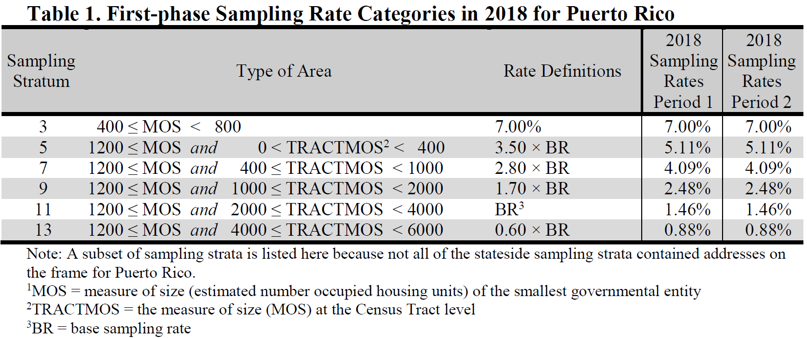
After each block is assigned to a second-stage sampling stratum in each period, a systematic sample of addresses is selected from the second-stage universe (first-stage sample) within each county and county equivalent.
After the second stage of sampling, addresses selected during Period 1 sampling that are not in remote Alaska are randomly assigned to one of the first six months of the sample year. Sample addresses selected during Period 2 sampling that are not in remote Alaska are randomly assigned to a month from July through December, inclusive. Sample addresses in remote Alaska are assigned to the January or September panel in Period 1 and Period 2 sampling, respectively.
The addresses from which CAPI sub-samples are selected can be divided into two groups. One group includes addresses that are not eligible for any other data collection operation - these consist of unmailable addresses and those in remote Alaska areas. The second group includes addresses that are eligible for the other data collection operations but for which no response was obtained prior to CAPI sub-sampling - these consist of mailable addresses not in a remote Alaska area.
All sample addresses in remote Alaska are sent to the CAPI data collection operation. Most unmailable addresses are selected for CAPI at a rate of 2-in-3 - the exception is when they are in a Hawaiian Homeland area (HH), Alaska Native Village Statistical area (ANVSA), or pre-determined American Indian areas (AI), where all are selected for CAPI.
With one exception, mailable addresses from which a response was not obtained by the time of the CAPI operation are sampled at rates of 1-in-2, 2-in-5, and 1-in-3 - these rates are set at the tract level. The exception is for addresses in HH, ANVSA, and AI areas, where all are selected for CAPI. Table 2 shows the CAPI sub-sampling rates that are associated with each group of addresses.
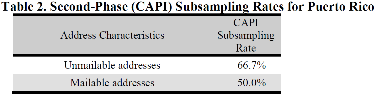
The 2019 group quarters (GQ) sampling frame was divided into two strata: a small GQ stratum and a large GQ stratum. Small GQs are defined to have expected populations of fifteen or fewer residents, while large GQs have expected populations of more than fifteen residents.
Samples were selected in two phases within each stratum. In general, GQs were selected in the first phase and then persons/residents were selected in the second phase. Both phases differ between the two strata. Each sampled GQ was randomly assigned to one or more months in 2019 - it was in these months that their person samples were selected.
Samples were selected in two phases within each stratum. In general, GQs were selected in the first phase and then persons/residents were selected in the second phase. Both phases differ between the two strata. Each sampled GQ was randomly assigned to one or more months in 2019 - it was in these months that their person samples were selected.
There were two stages of selecting small GQs for sample.
- First stage
The small GQ universe is divided into five groups that are approximately equal in size. All new small GQs are systematically assigned to one of these five groups on a yearly basis, with about the same probability (20 percent) of being assigned to any given group. Each group represents a second-stage sampling frame, from which GQs are selected once every five years. The 2019 secondstage sampling frame was used in 2013 as well, and is currently to be used in 2023, 2028, etc. - Second stage
GQs were systematically selected from the 2019 second-stage sampling frame. Each GQ had the same second-stage probability of being selected within a given state, where the probabilities varied between states. Table 3 below shows these probabilities.
Persons were selected for sample from each GQ that was selected for sample in the first phase of sample selection. If fifteen or fewer persons were residing at a GQ at the time a field representative (interviewer) visited the GQ, then all persons were selected for
sample. Otherwise, if more than fifteen persons were residing at the GQ, then the interviewer selected a systematic sample of ten persons from the GQ's roster.
The targeted state-level sampling rates are the probabilities of selecting any given person in a GQ; it is around these probabilities that the sample design is based. These probabilities reflect both phases of sample selection, and they varied by state. The
probabilities for 2019 are shown in Table 3.
The sample was designed so that the second-phase sampling rate would be one-hundred percent for small GQs (i.e., select the entire expected population of fifteen or fewer persons for sample in every small sampled GQ). This means the probability of selecting any person in a small GQ was designed to equal the probability of selecting the small GQ itself.
The sample was designed so that the second-phase sampling rate would be one-hundred percent for small GQs (i.e., select the entire expected population of fifteen or fewer persons for sample in every small sampled GQ). This means the probability of selecting any person in a small GQ was designed to equal the probability of selecting the small GQ itself.
All large GQs are eligible to be sampled as has been the case every year since the inception of the GQ sampling in 2006. This means there was only a single stage of sampling in this phase. This stage consists of systematically assigning "hits" to GQs
independently in each state, where each hit represents ten persons to be sampled.
In general, a GQ has either Z or Z+1 hits assigned to it. The value for Z is dependent on both the GQ's expected population size and its within-state target sampling rate, shown in Table 3. When this rate is multiplied by a GQ's expected population, the result is a GQ's expected person sample size. If a GQ's expected person sample size is less than ten, then Z = 0; if it is at least ten but less than twenty, then Z = 1; if it is at least twenty but less than thirty, then Z = 2; and so on. See below for a detailed example.
If a GQ has an expected person sample size that is less than ten, then this method effectively gives the GQ a probability of selection that is proportional to its size; this probability is the expected person sample size divided by ten. If a GQ has an expected person sample size of ten or more, then it is in sample with certainty and is assigned one or more hits.
In general, a GQ has either Z or Z+1 hits assigned to it. The value for Z is dependent on both the GQ's expected population size and its within-state target sampling rate, shown in Table 3. When this rate is multiplied by a GQ's expected population, the result is a GQ's expected person sample size. If a GQ's expected person sample size is less than ten, then Z = 0; if it is at least ten but less than twenty, then Z = 1; if it is at least twenty but less than thirty, then Z = 2; and so on. See below for a detailed example.
If a GQ has an expected person sample size that is less than ten, then this method effectively gives the GQ a probability of selection that is proportional to its size; this probability is the expected person sample size divided by ten. If a GQ has an expected person sample size of ten or more, then it is in sample with certainty and is assigned one or more hits.
Persons were selected within each GQ to which one or more hits were assigned in the first phase of selection. There were ten persons selected at a GQ for every hit assigned to the GQ. The persons were systematically sampled from a roster of persons residing at the GQ at the time of an interviewer's visit. The exception was if there were far fewer persons residing in a GQ than expected - in these situations, the number of persons to sample at the GQ would be reduced to reflect the GQ's actual population. In cases where
fewer than ten persons resided in a GQ at the time of a visit, the interviewer would select all of the persons for sample.
As for small GQs, the targeted sampling rate is the probability of selecting any given person in a GQ. This probability reflects both phases of sample selection. The targeted sampling rate for Puerto Rico in 2019 was 2.44 percent. Note that this is the same rate as
for persons in small GQs.
For example, suppose a GQ had an expected population of 500 and the targeted sampling rate was 2.26%- this means any given person in a GQ would have an approximately 1-in44.2478 chance of being selected. This rate, combined with the GQ's expected population of 500, means that the expected number of persons selected for sample in the GQ would be approximately 11.3 (2.26% x 500); this GQ would be assigned either one or two hits (Z = 1).
For example, suppose a GQ had an expected population of 500 and the targeted sampling rate was 2.26%- this means any given person in a GQ would have an approximately 1-in44.2478 chance of being selected. This rate, combined with the GQ's expected population of 500, means that the expected number of persons selected for sample in the GQ would be approximately 11.3 (2.26% x 500); this GQ would be assigned either one or two hits (Z = 1).
All sample GQs were assigned to one or more months (interview months) - these were the months in which interviewers would visit a GQ to select a person sample and conduct interviews. All small GQs, all large GQs that were assigned only one hit, all remote Alaska GQs, all sampled military facilities, and all sampled correctional facilities (regardless of how many hits a military or correctional facility was assigned) were assigned to a single interview month. Remote Alaska GQs were assigned to either January or September; Federal prisons were assigned to September; all of the others were randomly assigned one interview month.
All large GQs that had been assigned multiple hits, but were not in any of the categories above, had each hit randomly assigned to a different interview month. If a GQ had more than twelve hits assigned to it, then multiple hits would be assigned to one or more interview months for the GQ. For example, if a GQ had fifteen hits assigned to it, then there would be three interview months in which two hits were assigned and nine interview months in which one hit was assigned. There are two restrictions to this process. One restriction is applied to college dormitories, whose hits are randomly assigned to non-summer months only, i.e., January through April and September through December. The other restriction is applied to military ships, whose hits were randomly assigned only to the last ten months of the year, i.e., March through December.
All large GQs that had been assigned multiple hits, but were not in any of the categories above, had each hit randomly assigned to a different interview month. If a GQ had more than twelve hits assigned to it, then multiple hits would be assigned to one or more interview months for the GQ. For example, if a GQ had fifteen hits assigned to it, then there would be three interview months in which two hits were assigned and nine interview months in which one hit was assigned. There are two restrictions to this process. One restriction is applied to college dormitories, whose hits are randomly assigned to non-summer months only, i.e., January through April and September through December. The other restriction is applied to military ships, whose hits were randomly assigned only to the last ten months of the year, i.e., March through December.
Prior to 2016, all GQs were sampled at the same time for a given year. Starting in 2016, Bureau of Prison GQs (Federal prisons) started to be sampled separately from other GQs. They are sampled using the same procedure described above, and are all assigned to the September interview month as before.
Counts of sample addresses and GQ persons can be found in two locations on the US Census Bureau website. In American Fact Finder, base tables B98001 and B98002 provide sample size counts for the Puerto Rico and municipios. Sample size definitions and sample size counts for Puerto Rico are also available in the Sample Size and Data Quality Section of the ACS website, at https://www.census.gov/acs/www/methodology/sample-size-and-data-quality/.
Counts of sample addresses and GQ persons can be found in two locations on the US Census
Bureau website. On data.census.gov, base tables B98001 and B98002 provide sample size
counts for the Puerto Rico and municipios. Sample size definitions and sample size counts for
Puerto Rico are also available in the Sample Size and Data Quality Section of the ACS
website, at
https://www.census.gov/acs/www/methodology/sample-size-and-data-quality
The estimates that appear in this product are obtained from a raking ratio estimation procedure that results in the assignment of two sets of weights: a weight to each sample person record and a weight to each sample housing unit record. Estimates of person characteristics are based on the person weight. Estimates of family, household, and housing unit characteristics are based on the housing unit weight. For any given tabulation area, a characteristic total is estimated by summing the weights assigned to the persons, households, families or housing units possessing the characteristic in the tabulation area. Each sample person or housing unit record is assigned exactly one weight to be used to produce estimates of all characteristics. For example, if the weight given to a sample person or housing unit has a value 40, all characteristics of that person or housing unit are tabulated with the weight of 40.
The weighting is conducted in two main operations: a group quarters person weighting operation which assigns weights to persons in group quarters, and a household person weighting operation which assigns weights both to housing units and to persons within housing units. The group quarters person weighting is conducted first and the household person weighting second. The household person weighting is dependent on the group quarters person weighting because estimates for total population, which include both group quarters and household population, are controlled to the Census Bureau's official 2019 total resident population estimates.
The weighting is conducted in two main operations: a group quarters person weighting operation which assigns weights to persons in group quarters, and a household person weighting operation which assigns weights both to housing units and to persons within housing units. The group quarters person weighting is conducted first and the household person weighting second. The household person weighting is dependent on the group quarters person weighting because estimates for total population, which include both group quarters and household population, are controlled to the Census Bureau's official 2019 total resident population estimates.
Starting with the weighting for the 2011 1-year ACS estimates, the group quarters (GQ) person weighting changed in important ways from previous years' weighting. The GQ population sample was supplemented by a large-scale whole person imputation into not-in-sample GQ facilities. For the 2019 ACS GQ data, roughly as many GQ persons were imputed as interviewed. The goal of the imputation methodology was two-fold.
The GQ sampling frame was modified to create an imputation frame from which all imputed GQs were selected from. The frame was updated with the actual populations and GQ type changes from ACS interviews, as well as any subsequent information gathered in other processes since the sampling frame was initially created. The change in populations for ACS GQ interviews was used to calculate a not-in-sample adjustment factor that was used to update the population for all GQs on the frame not selected for sample. This adjustment factor was calculated at the following level:
GQ Major Type x GQ Size Stratum
There were three size strata used for this process: GQs in sample with certainty, GQs with 16 or more persons, and GQs with less than 16 persons.
For all not-in-sample GQ facilities with an expected population of 16 or more persons (large facilities), we imputed a number of GQ persons equal to 2.5% of the expected population. For those GQ facilities with an expected population of fewer than 16 persons (small facilities), we selected a random sample of GQ facilities as needed to accomplish the two objectives given above. For those selected small GQ facilities, we imputed a number of GQ persons equal to 20% of the facility's expected population.
Interviewed GQ person records were then sampled at random to be donors for the imputed persons of the selected not-in-sample GQ facilities. An expanding search algorithm searched for donors within the same specific type of GQ facility and the same county. If that failed, the search included all GQ facilities of the same major GQ type group. If that still failed, the search expanded to a specific type within state, then a major GQ type group within state. This expanding search continued through division, region, and the entire nation until suitable donors were found.
The weighting procedure made no distinction between sampled and imputed GQ person records. The initial weights of person records in the large GQ facilities equaled the observed or expected population of the GQ facility divided by the number of person records. The initial weights of person records in small GQ facilities equaled the observed or expected population of the GQ facility divided by the number of records, multiplied by the inverse of the fraction of small GQ facilities represented in the weighting to the number on the frame of that tract by major GQ type group combination.
The population totals on the imputation frame are used to ensure that the sub-state distribution of GQ weighting preserves the distribution from the frame. This accomplished through a series of three constraints:
Lastly, the final GQ person weight was rounded to an integer. Rounding was performed so that the sum of the rounded weights were within one person of the sum of the unrounded weights for any of the groups listed below:
Major GQ Type Group
Major GQ Type Group x Municipio
- The primary objective was to establish representation of municipio by major GQ type group in the tabulations for each combination that exists on the PRCS GQ sample frame. The seven major GQ type groups are defined by the Population Estimates Program and
are given in Table 3.
- A secondary objective was to establish representation of tract by major GQ type group for each combination that exists on the PRCS GQ sample frame.
The GQ sampling frame was modified to create an imputation frame from which all imputed GQs were selected from. The frame was updated with the actual populations and GQ type changes from ACS interviews, as well as any subsequent information gathered in other processes since the sampling frame was initially created. The change in populations for ACS GQ interviews was used to calculate a not-in-sample adjustment factor that was used to update the population for all GQs on the frame not selected for sample. This adjustment factor was calculated at the following level:
GQ Major Type x GQ Size Stratum
There were three size strata used for this process: GQs in sample with certainty, GQs with 16 or more persons, and GQs with less than 16 persons.
For all not-in-sample GQ facilities with an expected population of 16 or more persons (large facilities), we imputed a number of GQ persons equal to 2.5% of the expected population. For those GQ facilities with an expected population of fewer than 16 persons (small facilities), we selected a random sample of GQ facilities as needed to accomplish the two objectives given above. For those selected small GQ facilities, we imputed a number of GQ persons equal to 20% of the facility's expected population.
Interviewed GQ person records were then sampled at random to be donors for the imputed persons of the selected not-in-sample GQ facilities. An expanding search algorithm searched for donors within the same specific type of GQ facility and the same county. If that failed, the search included all GQ facilities of the same major GQ type group. If that still failed, the search expanded to a specific type within state, then a major GQ type group within state. This expanding search continued through division, region, and the entire nation until suitable donors were found.
The weighting procedure made no distinction between sampled and imputed GQ person records. The initial weights of person records in the large GQ facilities equaled the observed or expected population of the GQ facility divided by the number of person records. The initial weights of person records in small GQ facilities equaled the observed or expected population of the GQ facility divided by the number of records, multiplied by the inverse of the fraction of small GQ facilities represented in the weighting to the number on the frame of that tract by major GQ type group combination.
The population totals on the imputation frame are used to ensure that the sub-state distribution of GQ weighting preserves the distribution from the frame. This accomplished through a series of three constraints:
- Tract Constraint (TRCON) - This factor makes the total weight within each tract by major type group equal the total population from the imputation frame.
- County Constraint (CYCON) - This factor makes the total weight within each county by major type group equal the total population from the imputation frame.
- State Constraint (STCON) - This factor makes the total weight within each state by major type group equal the total population from the imputation frame.
Lastly, the final GQ person weight was rounded to an integer. Rounding was performed so that the sum of the rounded weights were within one person of the sum of the unrounded weights for any of the groups listed below:
Major GQ Type Group
Major GQ Type Group x Municipio
The housing unit and household person weighting uses two types of geographic areas for adjustments: weighting areas and subcounty areas. Weighting areas are county-based and have been used since the first year of the ACS. Subcounty areas are based on incorporated place and minor civil divisions (MCD). Their use was introduced into the ACS in 2010.
Weighting areas were built from collections of whole counties. The 2010 Census data and 2007-2011 ACS 5-year data were used to group counties of similar demographic and social characteristics. The characteristics considered in the formation included:
The estimation procedure used to assign the weights is then performed independently within each of the PRCS weighting areas.
Weighting areas were built from collections of whole counties. The 2010 Census data and 2007-2011 ACS 5-year data were used to group counties of similar demographic and social characteristics. The characteristics considered in the formation included:
- Percent in poverty (the only characteristic using ACS 5-year data)
- Percent renting
- Density of housing units (a proxy for rural areas)
- Race, ethnicity, age, and sex distribution
- Distance between the centroids of the counties
- Core-based Statistical Area status
The estimation procedure used to assign the weights is then performed independently within each of the PRCS weighting areas.
This process produced the following factors:
Base Weight (BW)
This initial weight is assigned to every housing unit as the inverse of its block’s sampling rate.
CAPI Subsampling Factor (SSF)
The weights of the CAPI cases are adjusted to reflect the results of CAPI subsampling.
This factor is assigned to each record as follows:
Selected in CAPI subsampling: SSF = 2.0, 2.5, or 3.0 according to Table 2
Not selected in CAPI subsampling: SSF = 0.0
Not a CAPI case: SSF = 1.0
Some sample addresses are unmailable. A two-thirds sample of these is sent directly to CAPI and for these cases SSF = 1.5.
Variation in Monthly Response by Mode (VMS)
This factor makes the total weight of the Mail, CATI, and CAPI records to be tabulated in a month equal to the total base weight of all cases originally mailed for that month. For all cases, VMS is computed and assigned based on the following groups:
Weighting Area x Month
Noninterview Factor (NIF)
This factor adjusts the weight of all responding occupied housing units to account for nonresponding housing units. The factor is a ratio adjustment that is computed and assigned to occupied housings units based on the following groups:
Weighting Area x Building Type (single or multi unit) x Tract
Vacant housing units are assigned a value of NIF = 1.0. Nonresponding housing units are assigned a weight of 0.0.
Initially the person weight of each person in an occupied housing unit is the product of the weighting factors of their associated housing unit (BW x ... x HPF). At this point, everyone in the household has the same weight. The person weighting is done in a series of three steps, which are repeated until a stopping criterion is met. These three steps form a raking ratio or raking process. These person weights are individually adjusted for each person as described below.
The three steps are as follows:
Municipio Controls Raking Factor (SUBEQRF)
TThis factor is applied to individuals based on their geography. It adjusts the person weights so that the weighted sample counts equal independent population estimates of total population for the municipio. For those municipios that are their own weighting area, this adjustment factor will be 1.0. Because of later adjustments to the person weights, total population is not assured of agreeing exactly with the official 2019 population estimates for municipios which are not their own weighting area.
Spouse Equalization/Householder Equalization Raking Factor (SPHHEQRF)
This factor is applied to individuals based on the combination of their status of being in a married-couple or unmarried-partner household and whether they are the householder.
All persons are assigned to one of four groups:
1. Householder in a married-couple or unmarried-partner household
2. Spouse or unmarried partner in a married-couple or unmarried-partner household (non-householder)
3. Other householder
4. Other non-householder
The weights of persons in the first two groups are adjusted so that their sums are each equal to the total estimate of married-couple or unmarried-partner households using the housing unit weight (BW x ... x HPF). At the same time, the weights of persons in the first and third groups are adjusted so that their sum is equal to the total estimate of occupied housing units using the housing unit weight (BW x ... x HPF). The goal of this step is to produce more consistent estimates of spouses or unmarried partners and married-couple and unmarried-partner households while simultaneously producing more consistent estimates of householders, occupied housing units, and households.
Demographic Raking Factor (DEMORF)
This factor is applied to individuals based on their age and sex in Puerto Rico (note that there are 13 Age groupings). It adjusts the person weights so that the weighted sample counts equal the independent population estimates by age and sex at the weighting area level. Because of collapsing of groups in applying this factor, only the total population is assured of agreeing with the official 2019 population estimates at the weighting area level.
These three steps are repeated several times until the estimates for Puerto Rico achieve their optimal consistency with regard to the spouse and householder equalization. The Person Post-Stratification Factor (PPSF) is then equal to the product (SUBEQRF x SPHHEQRF x DEMORF) from all of iterations of these three adjustments. The unrounded person weight is then the equal to the product of PPSF times the housing unit weight (BW x ... x MBF x PPSF).
The final product of all person weights (BW x ... x HPF x PPSF) is rounded to an integer.
Rounding is performed so that the sum of the rounded weights is within one person of the sum of the unrounded weights for any of the groups listed below:
Municipio
Municipio x Sex
Municipio x Sex x Age
Municipio x Sex x Age x Tract
Municipio x Sex x Age x Tract x Block
For example, the number of Males, Age 30 estimated for a municipio using the rounded weights is within one of the number produced using the unrounded weights.
This process produces the following factors:
Householder Factor (HHF)
This factor adjusts for differential response depending on the race, Hispanic origin, sex, and age of the householder. The value of HHF for an occupied housing unit is the PPSF of the householder. Since there is no householder for vacant units, the value of HHF = 1.0 for all vacant units.
Rounding
The final product of all housing unit weights (BW x ... x HHF) is rounded to an integer. For occupied units, the rounded housing unit weight is the same as the rounded person weight of the householder. This ensures that both the rounded and unrounded householder weights are equal to the occupied housing unit weight. The rounding for vacant housing units is then performed so that total rounded weight is within one housing unit of the total unrounded weight for any of the groups listed below:
Municipio
Municipio x Tract
Municipio x Tract x Block
The Census Bureau has modified or suppressed some data on this site to protect confidentiality. Title 13 United States Code, Section 9, prohibits the Census Bureau from publishing results in which an individual's data can be identified.
The Census Bureau's internal Disclosure Review Board sets the confidentiality rules for all data releases. A checklist approach is used to ensure that all potential risks to the confidentiality of the data are considered and addressed.
The Census Bureau's internal Disclosure Review Board sets the confidentiality rules for all data releases. A checklist approach is used to ensure that all potential risks to the confidentiality of the data are considered and addressed.
Title 13 of the United States Code authorizes the Census Bureau to conduct censuses and surveys. Section 9 of the same Title requires that any information collected from the public under the authority of Title 13 be maintained as confidential. Section 214 of Title 13 and Sections 3559 and 3571 of Title 18 of the United States Code provide for the imposition of penalties of up to five years in prison and up to $250,000 in fines for wrongful disclosure of confidential census information.
Disclosure avoidance is the process for protecting the confidentiality of data. A disclosure of data occurs when someone can use published statistical information to identify an individual who has provided information under a pledge of confidentiality. For data tabulations, the Census Bureau uses disclosure avoidance procedures to modify or remove the characteristics that put confidential information at risk for disclosure. Although it may appear that a table shows information about a specific individual, the Census Bureau has taken steps to disguise or suppress the original data while making sure the results are still useful. The techniques used by the Census Bureau to protect confidentiality in tabulations vary, depending on the type of data. All disclosure avoidance procedures are done prior to the whole person imputation into not-insample GQ facilities.
Data swapping is a method of disclosure avoidance designed to protect confidentiality in tables of frequency data (the number or percent of the population with certain characteristics). Data swapping is done by editing the source data or exchanging records for a sample of cases when creating a table. A sample of households is selected and matched on a set of selected key variables with households in neighboring geographic areas that have similar characteristics (such as the same number of adults and same number of children). Because the swap often occurs within a neighboring area, there is no effect on the marginal totals for the area or for totals that include data from multiple areas. Because of data swapping, users should not assume that tables with cells having a value of one or two reveal information about specific individuals. Data swapping procedures were first used in the 1990 Census, and were used again in Census 2000 and the 2010 Census.
The goals of using synthetic data are the same as the goals of data swapping, namely to protect the confidentiality in tables of frequency data. Persons are identified as being at risk for disclosure based on certain characteristics. The synthetic data technique then models the values for another collection of characteristics to protect the confidentiality of that individual.
The data in PRCS products are estimates of the actual figures that would be obtained by interviewing the entire population. The estimates are a result pf the chosen sample, and are subject to sample-to-sample variation. Sampling error in data arises due to the use of
probability sampling, which is necessary to ensure the integrity and representativeness of sample survey results. The implementation of statistical sampling procedures provides the basis for the statistical analysis of sample data. Measures used to estimate the sampling error are provided in the next section.
Other types of errors might be introduced during any of the various complex operations used to collect and process survey data. For example, data entry from questionnaires and editing may introduce error into the estimates. Another potential source of error is the use of controls in the weighting. These controls are based on Population Estimates and are designed to reduce variance and mitigate the effects of systematic undercoverage of groups who are difficult to enumerate. However, if the extrapolation methods used in generating the Population Estimates do not properly reflect the population, error can be introduced into the data. This potential risk is offset by the many benefits that the controls provide to the PRCS estimates, including the reduction of issues with survey coverage and the reduction of standard errors of PRCS estimates. These and other sources of error contribute to the nonsampling error component of the total error of survey estimates.
Nonsampling errors may affect the data in two ways. Errors that are introduced randomly increase the variability of the data. Systematic errors, or errors that consistently skew the data in one direction, introduce bias into the results of a sample survey. The Census Bureau protects against the effect of systematic errors on survey estimates by conducting extensive research and evaluation programs on sampling techniques, questionnaire design, and data collection and processing procedures.
An important goal of the PRCS is to minimize the amount of nonsampling error introduced through nonresponse for sample housing units. One way of accomplishing this is by following up on mail nonrespondents during the CATI and CAPI phases. For more information, see the section entitled "Control of Nonsampling Error".
Sampling error is the difference between an estimate based on a sample and the corresponding value that would be obtained if the estimate were based on the entire population (as from a census). Note that sample-based estimates will vary depending on the particular sample selected from the population. Measures of the magnitude of sampling error reflect the variation in the estimates over all possible samples that could have been selected from the population using the same sampling methodology.
Estimates of the magnitude of sampling errors - in the form of margins of error - are provided with all published PRCS data. The Census Bureau recommends that data users incorporate margins of error into their analyses, as sampling error in survey estimates could impact the conclusions drawn from the results.
Estimates of the magnitude of sampling errors - in the form of margins of error - are provided with all published PRCS data. The Census Bureau recommends that data users incorporate margins of error into their analyses, as sampling error in survey estimates could impact the conclusions drawn from the results.
A sample estimate and its estimated standard error may be used to construct confidence intervals about the estimate. These intervals are ranges that will contain the average value of the estimated characteristic that results over all possible samples, with a known probability.
For example, if all possible samples that could result under the ACS sample design were independently selected and surveyed under the same conditions, and if the estimate and its estimated standard error were calculated for each of these samples, then:
For example, if all possible samples that could result under the ACS sample design were independently selected and surveyed under the same conditions, and if the estimate and its estimated standard error were calculated for each of these samples, then:
- Approximately 68 percent of the intervals from one estimated standard error below the estimate to one estimated standard error above the estimate would contain the average result from all possible samples.
- Approximately 90 percent of the intervals from 1.645 times the estimated standard error below the estimate to 1.645 times the estimated standard error above the estimate would contain the average result from all possible samples.
- Approximately 95 percent of the intervals from two estimated standard errors below the estimate to two estimated standard errors above the estimate would contain the average result from all possible samples.
In lieu of providing upper and lower confidence bounds in published ACS tables, the margin of error is listed. All ACS published margins of error are based on a 90 percent confidence level. The margin of error is the difference between an estimate and its upper or lower confidence bound. Both the confidence bounds and the standard error can easily be computed from the margin of error:
Standard Error = Margin of Error / 1.645
Lower Confidence Bound = Estimate - Margin of Error
Upper Confidence Bound = Estimate + Margin of Error
Note that for 2005, PRCS margins of error and confidence bounds were calculated using a 90 percent confidence level multiplier of 1.65. Starting with the 2006 data release, and for every year after 2006, the more accurate multiplier of 1.645 is used. Margins of error and confidence bounds from previously published products will not be updated with the new multiplier. When calculating standard errors from margins of error or confidence bounds using published data for 2005, use the 1.65 multiplier When constructing confidence bounds from the margin of error, users should be aware of any "natural" limits on the bounds. For example, if a characteristic estimate for the population is near zero, the calculated value of the lower confidence bound may be negative. However, as a negative number of people does not make sense, the lower confidence bound should be reported as zero. For other estimates such as income, negative values can make sense; in these cases, the lower bound should not be adjusted. The context and meaning of the estimate must therefore be kept in mind when creating these bounds. Another example of a natural limit is 100 percent as the upper bound of a percent estimate.
If the margin of error is displayed as '*****' (five asterisks), the estimate has been controlled to be equal to a fixed value and so it has no sampling error. A standard error of zero should be used for these controlled estimates when completing calculations, such as those in the following section.
Users should be careful when computing and interpreting confidence intervals.
The estimated standard errors (and thus margins of error) included in these data products do not account for variability due to nonsampling error that may be present in the data. In particular, the standard errors do not reflect the effect of correlated errors introduced by interviewers, coders, or other field or processing personnel or the effect of imputed values due to missing responses. The standard errors calculated are only lower bounds of the total error. As a result, confidence intervals formed using these estimated standard errors may not meet the stated levels of confidence (i.e., 68, 90, or 95 percent). Some care must be exercised in the interpretation of the data based on the estimated standard errors.
By definition, the value of almost all PRCS characteristics is greater than or equal to zero. The method provided above for calculating confidence intervals relies on large sample theory, and may result in negative values for zero or small estimates for which negative
values are not admissible. In this case, the lower limit of the confidence interval should be set to zero by default. A similar caution holds for estimates of totals close to a control total or estimated proportion near one, where the upper limit of the confidence interval is set to its
largest admissible value. In these situations, the level of confidence of the adjusted range of values is less than the prescribed confidence level.
Direct estimates of margin of error were calculated for all estimates reported. The margin of error is derived from the variance. In most cases, the variance is calculated using a replicatebased methodology known as successive difference replication (SDR) that takes into account the sample design and estimation procedures.
The SDR formula as well as additional information on the formation of the replicate weights, can be found in Chapter 12 of the Design and Methodology documentation at: https://www.census.gov/programs-surveys/acs/methodology/design-and-methodology.html.
Beginning with the PRCS 2011 1-year estimates, a new imputation-based methodology was incorporated into processing (see the description in the Group Quarters Person Weighting Section). An adjustment was made to the production replicate weight variance methodology to account for the non-negligible amount of additional variation being introduced by the new technique.4
Excluding the base weights, replicate weights were allowed to be negative in order to avoid underestimating the standard error. Exceptions include:
Footnotes:
4For more information regarding this issue, see Asiala, M. and Castro, E. 2012. Developing Replicate WeightBased Methods to Account for Imputation Variance in a Mass Imputation Application. In JSM proceedings, Section on Survey Research Methods, Alexandria, VA: American Statistical Association.
The SDR formula as well as additional information on the formation of the replicate weights, can be found in Chapter 12 of the Design and Methodology documentation at: https://www.census.gov/programs-surveys/acs/methodology/design-and-methodology.html.
Beginning with the PRCS 2011 1-year estimates, a new imputation-based methodology was incorporated into processing (see the description in the Group Quarters Person Weighting Section). An adjustment was made to the production replicate weight variance methodology to account for the non-negligible amount of additional variation being introduced by the new technique.4
Excluding the base weights, replicate weights were allowed to be negative in order to avoid underestimating the standard error. Exceptions include:
- The estimate of the number or proportion of people, households, families, or housing units in a geographic area with a specific characteristic is zero. A special procedure is used to estimate the standard error.
- There are either no sample observations available to compute an estimate or standard error of a median, an aggregate, a proportion, or some other ratio, or there are too few sample observations to compute a stable estimate of the standard error. The estimate is represented in the tables by "-" and the margin of error by "**" (two asterisks).
- The estimate of a median falls in the lower open-ended interval or upper open-ended interval of a distribution. If the median occurs in the lowest interval, then a "-" follows the estimate, and if the median occurs in the upper interval, then a "+" follows the estimate. In both cases, the margin of error is represented in the tables by "***" (three asterisks).
Footnotes:
4For more information regarding this issue, see Asiala, M. and Castro, E. 2012. Developing Replicate WeightBased Methods to Account for Imputation Variance in a Mass Imputation Application. In JSM proceedings, Section on Survey Research Methods, Alexandria, VA: American Statistical Association.
Previously, this document included formulas for approximating the standard error (SE) for various types of estimates. For example, summing estimates or calculating a ratio of two or more estimates. These formulas are also found in the Instruction for Statistical Testing documents, which is located at https://www.census.gov/programs-surveys/acs/technicaldocumentation/code-lists.html. In addition, the worked examples have also been placed in the same location in the document called "Worked Examples for Approximating Margins of Error".
Users may conduct a statistical test to see if the difference between an PRCS estimate and any other chosen estimate is statistically significant at a given confidence level. "Statistically significant" means that it is not likely that the difference between estimates is due to random chance alone.
To perform statistical significance testing, data users will need to calculate a Z statistic. The equation is available in the Instructions for Statistical Testing, which is located at https://www.census.gov/programs-surveys/acs/technical-documentation/code-lists.html.
Users completing statistical testing may be interested in using the ACS Statistical Testing Tool.
This automated tool allows users to input pairs and groups of estimates for comparison. For more information on the Statistical Testing Tool, visit https://www.census.gov/programssurveys/acs/guidance/statistical-testing-tool.html.
As mentioned earlier, sample data are subject to nonsampling error. Nonsampling error can introduce serious bias into the data, increasing the total error dramatically over that which would result purely from sampling. While it is impossible to completely eliminate nonsampling error from a survey operation, the Census Bureau attempts to control the sources of such error during the collection and processing operations. Described below are the primary sources of nonsampling error and the programs instituted to control for this error.5
Footnotes:
5The success of these programs is contingent upon how well the instructions were carried out during the survey.
Footnotes:
5The success of these programs is contingent upon how well the instructions were carried out during the survey.
It is possible for some sample housing units or persons to be missed entirely by the survey (undercoverage). It is also possible for some sample housing units and persons to be counted more than once (overcoverage). Both undercoverage and overcoverage of persons and housing units can introduce bias into the data. Coverage error can also increase both respondent burden and survey costs.
To avoid coverage error in a survey, the frame must be as complete and accurate as possible. For the ACS, the frame is an address list in each state, the source of which is the Master Address File (MAF). An attempt is made to assign each MAF address to the appropriate geographic codes via an automated procedure using the Census Bureau TIGER (Topologically Integrated Geographic Encoding and Referencing) files. A manual coding operation based in the appropriate regional offices is attempted for addresses that could not be automatically coded.
In 2019, the MAF was used as the source of addresses for selecting sample housing units and mailing questionnaires. TIGER produced the location maps for CAPI assignments. Sometimes the MAF contains duplicates of addresses. This could occur when there is a slight difference in the address such as 123 Main Street versus 123 Maine Street, and can introduce overcoverage.
In the CATI and CAPI nonresponse follow-up phases, efforts were made to minimize the chances that housing units that were not part of the sample were mistakenly interviewed instead of units in sample. If a CATI interviewer called a mail nonresponse case and was not able to reach the exact address, no interview was conducted and the case became eligible for CAPI. During the CAPI follow-up, the interviewer had to locate the exact address for each sample housing unit. If the interviewer could not locate the exact sample unit in a multi-unit structure, or found a different number of units than expected, the interviewers were instructed to list the units in the building and follow a specific procedure to select a replacement sample unit. Person overcoverage can occur when an individual is included as a member of a housing unit but does not meet PRCS residency rules.
Coverage rates give a measure of undercoverage or overcoverage of persons or housing units in a given geographic area. Rates below 100 percent indicate undercoverage, while rates above 100 percent indicate overcoverage. Coverage rates are released concurrent with the release of estimates on data.census.gov6 in the B98 series of detailed tables (Table IDs B98011, B98012, B98013, and B980014). Coverage rate definitions and coverage rates for total population for Puerto Rico are also available in the Sample Size and Data Quality Section of the ACS website, at https://www.census.gov/acs/www/methodology/sample-size-and-data-quality/.
Footnotes:
6Beginning in 2019, data.census.gov replaces American Factfinder as the dissemination tool for publishing ACS tables and other data products.
Survey nonresponse is a well-known source of nonsampling error. There are two types of nonresponse error - unit nonresponse and item nonresponse. Nonresponse errors affect survey estimates to varying levels depending on amount of nonresponse and the extent to which the characteristics of nonrespondents differ from those of respondents. The exact amount of nonresponse error or bias on an estimate is almost never known. Therefore, survey researchers generally rely on proxy measures, such as the nonresponse rate, to indicate the potential for nonresponse error.
Unit nonresponse is the failure to obtain data from housing units in the sample. Unit nonresponse may occur because households are unwilling or unable to participate, or because an interviewer is unable to make contact with a housing unit. Unit nonresponse is
problematic when there are systematic or variable differences in the characteristics of interviewed and non-interviewed housing units. Nonresponse bias is introduced into an estimate when differences are systematic; the nonresponse error of an estimate evolves from variable differences between interviewed and non-interviewed households.
The PRCS made every effort to minimize unit nonresponse, and thus, the potential for nonresponse error. First, the PRCS used a combination of mail, CATI, and CAPI data collection modes to maximize response. The mail phase included a series of three to four mailings to encourage housing units to return the questionnaire. Subsequently, mail nonrespondents (for which phone numbers are available) were contacted by CATI for an interview. Finally, a subsample of the mail and telephone nonrespondents was contacted for by personal visit to attempt an interview
PRCS response rates measure the percent of units with a completed interview. The higher the response rate (and, consequently, the lower the nonresponse rate), the lower the chance that estimates are affected by nonresponse bias. Response and nonresponse rates, as well as rates for specific types of nonresponse, are released concurrent with the release of estimates on data.census.gov7 in the B98 series of detailed tables (Table IDs B98021and B98022). Unit response rate definitions and unit response rates by type for Puerto Rico are also available in the Sample Size and Data Quality Section of the ACS website, athttps://www.census.gov/acs/www/methodology/sample-size-and-data-quality/.
Footnotes:
7Beginning in 2019, data.census.gov replaces American Factfinder as the dissemination tool for publishing ACS tables and other data products.
Nonresponse to particular questions on the survey can introduce error or bias into the data, as
the unknown characteristics of nonrespondents may differ from those of respondents. As a
result, any imputation procedure using respondent data may not completely reflect difference
either at the elemental level (individual person or housing unit) or on average.
Some protection against the introduction of large errors or biases is afforded by minimizing nonresponse. In the PRCS, item nonresponse for the CATI and CAPI operations was minimized by requiring that the automated instrument receive a response to each question before the next question could be asked. Questionnaires returned by mail were reviewed by computer for content omissions and population coverage and edited for completeness and acceptability. They were. If necessary, a telephone follow-up was made to obtain missing information. Potential coverage errors were included in this follow-up.
Potential coverage errors were included in this follow-up.
Allocation tables provide the weighted estimate of persons or housing units for which a value was imputed, as well as the total estimate of persons or housing units that were eligible to answer the question. The smaller the number of imputed responses, the lower the chance that the item nonresponse is contributing a bias to the estimates. Allocation tables are released concurrent with the release of estimates on data.census.gov8 in the B99 series of detailed tables with the overall allocation rates across all person and housing unit characteristics in the B98 series of detailed tables (Table IDs B98031 and B98032). Allocation rate definitions and allocation rates by characteristic for Puerto Rico are also available in the Sample Size and Data Quality Section of the ACS website, at https://www.census.gov/acs/www/methodology/sample-size-and-data-quality/.
Footnotes:
8Beginning in 2019, data.census.gov replaces American Factfinder as the dissemination tool for publishing ACS tables and other data products.
Measurement error can arise if the person completing the questionnaire or responding an interviewer's questions responds incorrectly. However, to mitigate this risk, the phrasing survey questions underwent cognitive testing and households were provided detailed instructions on how to complete the questionnaire.
Processing error can be introduced in numerous areas during data collection and capture, including during interviews, during data processing and during content editing
Processing error can be introduced in numerous areas during data collection and capture, including during interviews, during data processing and during content editing
An interviewer could introduce error by:
- Misinterpreting or otherwise incorrectly entering information given by a respondent.
- Failing to collect some of the information for a person or household.
- Collecting data for households that were not designated as part of the sample.
The many phases involved in processing the survey data represent potential sources for the introduction of nonsampling error. The processing of the survey questionnaires includes the keying of data from completed questionnaires, automated clerical review, follow-up by telephone, manual coding of write-in responses, and automated data processing. The various field, coding and computer operations undergo a number of quality control checks to insure their accurate application.
After data collection was completed, any remaining incomplete or inconsistent information was imputed during the final content edit of the collected data. Imputations, or computer assignments of acceptable codes in place of unacceptable entries or blanks, were most often needed either when an entry for a given item was missing or when information reported for a person or housing unit was inconsistent with other information for the same person or housing unit. As in other surveys and previous censuses, unacceptable entries were to allocated entries for persons or housing units with similar characteristics. Imputing acceptable values in place of blanks or unacceptable entries enhances the usefulness of the data.

