


| Documentation: | ACS 2013 (1-Year Estimates) |
you are here:
choose a survey
survey
document
chapter
Publisher: U.S. Census Bureau
Survey: ACS 2013 (1-Year Estimates)
| Document: | ACS 2013-1yr Summary File: Technical Documentation |
| citation: | Social Explorer; U.S. Census Bureau; American Community Survey 2013 Summary File: Technical Documentation. |
Chapter Contents
ACS 2013-1yr Summary File: Technical Documentation
The data contained in these data products are based on the American Community Survey (ACS) sample interviewed from January 1, 2013 through December 31, 2013. The ACS sample is selected from all counties and county-equivalents in the United States. In 2006, the ACS began collection of data from sampled persons in group quarters (GQs) – for example, military barracks, college dormitories, nursing homes, and correctional facilities. Persons in group quarters are included with persons in housing units (HUs) in all 2013 ACS estimates that are based on the total population. All ACS population estimates from years prior to 2006 include only persons in housing units. The ACS, like any other statistical activity, is subject to error. The purpose of this documentation is to provide data users with a basic understanding of the ACS sample design, estimation methodology, and accuracy of the ACS data. The ACS is sponsored by the U.S. Census Bureau, and is part of the Decennial Census Program.
Additional information on the design and methodology of the ACS, including data collection and processing, can be found at:: http://www.census.gov/acs/www/methodology/methodology_main/.
The 2013 Accuracy of the Data from the Puerto Rico Community Survey can be found at
http://www.census.gov/acs/www/Downloads/data_documentation/Accuracy/PRCS_Accuracy_of_Data_2013.pdf.
Housing Units
The ACS employs three modes of data collection:
Month 1: Addresses in sample that are determined to be mailable are sent an initial mailing package – this package contains information for completing the ACS questionnaire on the internet (on-line). If, after two weeks, a sample address has not responded on-line, then it is sent a second mailing package. This package contains a paper questionnaire. Once the second package is received, sampled addresses then have the option of which mode to use for filling out the questionnaire.
Month 2: All mail non-responding addresses with an available phone number are sent to CATI.
Month 3: A sample of mail non-responses without a phone number, CATI non-responses, and unmailable addresses are selected and sent to CAPI.
Note that mail responses are accepted during all three months of data collection.
All Remote Alaska addresses that are in sample are assigned to one of two data collection periods, January-April, or September-December and are all sent to the CAPI mode of data collection.1 Data for these addresses are collected using CAPI only and up to four months are given to complete the interviews in Remote Alaska for each data collection period.
1 Prior to the 2011 sample year, all remote Alaska sample cases were subsampled for CAPI at a rate of 2-in-3.
The ACS employs three modes of data collection:
- Internet
- Mailout/Mailback
- Computer Assisted Telephone Interview (CATI)
- Computer Assisted Personal Interview (CAPI)
Month 1: Addresses in sample that are determined to be mailable are sent an initial mailing package – this package contains information for completing the ACS questionnaire on the internet (on-line). If, after two weeks, a sample address has not responded on-line, then it is sent a second mailing package. This package contains a paper questionnaire. Once the second package is received, sampled addresses then have the option of which mode to use for filling out the questionnaire.
Month 2: All mail non-responding addresses with an available phone number are sent to CATI.
Month 3: A sample of mail non-responses without a phone number, CATI non-responses, and unmailable addresses are selected and sent to CAPI.
Note that mail responses are accepted during all three months of data collection.
All Remote Alaska addresses that are in sample are assigned to one of two data collection periods, January-April, or September-December and are all sent to the CAPI mode of data collection.1 Data for these addresses are collected using CAPI only and up to four months are given to complete the interviews in Remote Alaska for each data collection period.
1 Prior to the 2011 sample year, all remote Alaska sample cases were subsampled for CAPI at a rate of 2-in-3.
Group Quarters data collection spans six weeks, except in Remote Alaska and for Federal prisons, where the data collection time period is four months. As is done for housing unit (HU) addresses, Group Quarters in Remote Alaska are assigned to one of two data collection periods, January-April, or September-December and up to four months is allowed to complete the interviews. Similarly, all Federal prisons are assigned to September with a four month data collection window.
Field representatives have several options available to them for data collection. These include completing the questionnaire while speaking to the resident in person or over the telephone, conducting a personal interview with a proxy, such as a relative or guardian, or leaving paper questionnaires for residents to complete for themselves and then pick them up later. This last option is used for data collection in Federal prisons.
Field representatives have several options available to them for data collection. These include completing the questionnaire while speaking to the resident in person or over the telephone, conducting a personal interview with a proxy, such as a relative or guardian, or leaving paper questionnaires for residents to complete for themselves and then pick them up later. This last option is used for data collection in Federal prisons.
The universe for the ACS consists of all valid, residential housing unit addresses in all county and county equivalents in the 50 states, including the District of Columbia. The Master Address File (MAF) is a database maintained by the Census Bureau containing a listing of residential and commercial addresses in the U.S. and Puerto Rico. The MAF is updated twice each year with the Delivery Sequence Files (DSF) provided by the U.S. Postal Service. The DSF covers only the U.S. These files identify mail drop points and provide the best available source of changes and updates to the housing unit inventory. The MAF is also updated with the results from various Census Bureau field operations, including the ACS.
As in previous years, due to operational difficulties associated with data collection, the ACS excludes certain types of GQs from the sampling universe and data collection operations. The weighting and estimation accounts for this segment of the population included in the population controls. The following GQ types were removed from the GQ universe:
- Soup kitchens
- Domestic violence shelters
- Regularly scheduled mobile food vans
- Targeted non-sheltered outdoor locations
- Maritime/merchant vessels
- Living quarters for victims of natural disasters
- Dangerous encampments
The ACS employs a two-phase, two-stage sample design. The ACS first-phase sample consists of two separate samples, Main and Supplemental, each chosen at different points in time. Together, these constitute the first-phase sample. Both the Main and the Supplemental samples are chosen in two stages referred to as first- and second-stage sampling. Subsequent to second- stage sampling, sample addresses are randomly assigned to one of the twelve months of the sample year. The second-phase of sampling occurs when the CAPI sample is selected (see Section 2 below).
The Main sample is selected during the summer preceding the sample year. Approximately 99 percent of the sample is selected at this time. Each address in sample is randomly assigned to one of the 12 months of the sample year. Supplemental sampling occurs in January/February of the sample year and accounts for approximately 1 percent of the overall first-phase sample. The Supplemental sample is allocated to the last six months of the sample year. A sub-sample of non-responding addresses and of any addresses deemed unmailable is selected for the CAPI data collection mode2.
Several steps used to select the first-phase sample are common to both Main and Supplemental sampling. The descriptions of the steps included in the first-phase sample selection below indicate which are common to both and which are unique to either Main or Supplemental sampling.
1. First-phase Sample Selection
- Counties
- Places
- School Districts (elementary, secondary, and unified)
- American Indian Areas
- Tribal Subdivisions
- Alaska Native Village Statistical Areas
- Hawaiian Homelands
- Minor Civil Divisions - in Connecticut, Maine, Massachusetts, Michigan, Minnesota, New Hampshire, New Jersey, New York, Pennsylvania, Rhode Island, Vermont, and Wisconsin (these are the states where MCDs are active, functioning governmental units)
- Census Designated Places - in Hawaii only
The measure of size for all areas except American Indian Areas, Tribal Subdivisions, and Alaska Native Village Statistical Areas is an estimate of the number of occupied HUs in the area. This is calculated by multiplying the number of ACS addresses by an estimated occupancy rate at the block level. A measure of size for each Census Tract is also calculated in the same manner.
For American Indian, Tribal Subdivisions, and Alaska Native Village Statistical Areas, the measure of size is the estimated number of occupied HUs multiplied by the proportion of people reporting American Indian or Alaska Native (alone or in combination) in the 2010 Census.
Each block is then assigned the smallest positive, non-zero measure of size from the set of all entities of which it is a part. The 2013 second-stage sampling strata and the overall first-phase sampling rates are shown in Table 1 below. The sample rates represent the actual percent in sample that was delivered for the 2013 sample year.
Table 1. First-phase Sampling Rate Categories for the United States
2. Second-phase Sample Selection - Subsampling the Unmailable and Non-Responding Addresses
Most addresses determined to be unmailable are subsampled for the CAPI phase of data collection at a rate of 2-in-3. Unmailable addresses, which include Remote Alaska addresses, do not go to the CATI phase of data collection. Subsequent to CATI, all addresses for which no response has been obtained prior to CAPI are subsampled based on the expected rate of completed interviews at the tract level using the rates shown in Table 2.
Table 2. Second-Phase (CAPI) Subsampling Rates for the United States
2Beginning with the August, 2011 CAPI sample all non-mailable and non-responding addresses in the following areas are now sent to CAPI: all Hawaiian Homelands, all Alaska Native Village Statistical areas, American Indian areas with an estimated proportion of American Indian population ≥ 10%.
3Beginning with the 2011 sample the ACS implemented a change to the stratification, increasing the number of sampling strata and changing how the sampling rates are defined. Prior to 2011 there were seven strata, there are now 16 sampling strata. Table 1 gives a summary of these strata and the rates.
4The annual target sample size for the ACS was increased to the 3.54 million level beginning with the June, 2011 panel. Therefore, the U.S sample size increased from roughly 242,000 per month to 295,000 per month starting with the June, 2011 mail-out. The final 2011 sample was 3,272,520. The annual target sample size remains at 3.54 million.
The Main sample is selected during the summer preceding the sample year. Approximately 99 percent of the sample is selected at this time. Each address in sample is randomly assigned to one of the 12 months of the sample year. Supplemental sampling occurs in January/February of the sample year and accounts for approximately 1 percent of the overall first-phase sample. The Supplemental sample is allocated to the last six months of the sample year. A sub-sample of non-responding addresses and of any addresses deemed unmailable is selected for the CAPI data collection mode2.
Several steps used to select the first-phase sample are common to both Main and Supplemental sampling. The descriptions of the steps included in the first-phase sample selection below indicate which are common to both and which are unique to either Main or Supplemental sampling.
1. First-phase Sample Selection
- First-stage sampling (performed during both Main and Supplemental sampling) - First stage sampling defines the universe for the second stage of sampling through two steps. First, all addresses that were in a first-phase sample within the past four years are excluded from eligibility. This ensures that no address is in sample more than once in any five-year period. The second step is to select a 20 percent systematic sample of "new" units, i.e. those units that have never appeared on a previous MAF extract. Each new address is systematically assigned to either the current year or to one of four back- samples. This procedure maintains five equal partitions (samples) of the universe.
- Assignment of blocks to a second-stage sampling stratum (performed during Main sampling only) - Second-stage sampling uses 16 sampling strata in the U.S3. The stratum level rates used in second-stage sampling account for the first-stage selection probabilities. These rates are applied at a block level to addresses in the U.S. by calculating a measure of size for each of the following geographic entities:
- Counties
- Places
- School Districts (elementary, secondary, and unified)
- American Indian Areas
- Tribal Subdivisions
- Alaska Native Village Statistical Areas
- Hawaiian Homelands
- Minor Civil Divisions - in Connecticut, Maine, Massachusetts, Michigan, Minnesota, New Hampshire, New Jersey, New York, Pennsylvania, Rhode Island, Vermont, and Wisconsin (these are the states where MCDs are active, functioning governmental units)
- Census Designated Places - in Hawaii only
The measure of size for all areas except American Indian Areas, Tribal Subdivisions, and Alaska Native Village Statistical Areas is an estimate of the number of occupied HUs in the area. This is calculated by multiplying the number of ACS addresses by an estimated occupancy rate at the block level. A measure of size for each Census Tract is also calculated in the same manner.
For American Indian, Tribal Subdivisions, and Alaska Native Village Statistical Areas, the measure of size is the estimated number of occupied HUs multiplied by the proportion of people reporting American Indian or Alaska Native (alone or in combination) in the 2010 Census.
Each block is then assigned the smallest positive, non-zero measure of size from the set of all entities of which it is a part. The 2013 second-stage sampling strata and the overall first-phase sampling rates are shown in Table 1 below. The sample rates represent the actual percent in sample that was delivered for the 2013 sample year.
- Calculation of the second-stage sampling rates (performed during Main sampling only) - The overall first-phase sampling rates given in Table 1 are calculated using the distribution of ACS valid addresses by second-stage sampling stratum in such a way as to yield an overall target sample size for the year of 3,540,000 in the U.S. These rates also account for expected growth of the HU inventory between Main and Supplemental of roughly 1 percent. The first-phase rates are adjusted for the first-stage sample to yield the second-stage selection probabilities4.
- Second-stage sample selection (performed in Main and Supplemental) - After each block is assigned to a second-stage sampling stratum, a systematic sample of addresses is selected from the second-stage universe (first-stage sample) within each county and county equivalent.
- Sample Month Assignment (performed in Main and Supplemental) - After the second stage of sampling, all sample addresses are randomly assigned to a sample month. Addresses selected during Main sampling are allocated to each of the 12 months. Addresses selected during Supplemental sampling are assigned to the months of July through December.
Table 1. First-phase Sampling Rate Categories for the United States
| Sampling Stratum | Type of Area | Rate Definitions | 2013 Sampling Rate |
| 1 | 0 < MOS1 ≤ 200 | 15% | 15.00% |
| 2 | 200 < MOS ≤ 400 | 10% | 10.00% |
| 3 | 400 < MOS ≤ 800 | 7% | 7.00% |
| 4 | 800 < MOS ≤ 1,200 | 2.8 × BR | 4.40% |
| 5 | 0 < TRACTMOS2 ≤ 400 | 3.5 × BR | 5.55% |
| 6 | 0 < TRACTMOS ≤ 400 H.R.3 | 0.92 × 3.5 × BR | 5.06% |
| 7 | 400 < TRACTMOS ≤ 1,000 | 2.8 × BR | 4.40% |
| 8 | 400 < TRACTMOS ≤ 1,000 H.R. | 0.92 × 2.8 × BR | 4.04% |
| 9 | 1,000 < TRACTMOS ≤ 2,000 | 1.7 × BR | 2.67% |
| 10 | 1,000 < TRACTMOS ≤ 2,000 H.R. | 0.92 × 1.7 × BR | 2.46% |
| 11 | 2,000 < TRACTMOS ≤ 4,000 | BR4 | 1.57% |
| 12 | 2,000 < TRACTMOS ≤ 4,000 H.R. | 0.92 × BR | 1.44% |
| 13 | 4,000 < TRACTMOS ≤ 6,000 | 0.6 × BR | 0.94% |
| 14 | 4,000 < TRACTMOS ≤ 6,000 H.R. | 0.92 × 0.6 × BR | 0.87% |
| 15 | 6,000 < TRACTMOS | 0.35 × BR | 0.55% |
| 16 | 6,000 < TRACTMOS H.R. | 0.92 × 0.35 × BR | 0.51% |
| 1MOS = measure of size (estimated number occupied housing units) of the smallest governmental entity | |||
| 2TRACTMOS = the measure of size (MOS) at the Census Tract level | |||
| 3H.R. = areas where predicted levels of completed mail and CATI interviews are > 60% | |||
| 4BR = base sampling rate | |||
| 5NA = not applicable | |||
2. Second-phase Sample Selection - Subsampling the Unmailable and Non-Responding Addresses
Most addresses determined to be unmailable are subsampled for the CAPI phase of data collection at a rate of 2-in-3. Unmailable addresses, which include Remote Alaska addresses, do not go to the CATI phase of data collection. Subsequent to CATI, all addresses for which no response has been obtained prior to CAPI are subsampled based on the expected rate of completed interviews at the tract level using the rates shown in Table 2.
Table 2. Second-Phase (CAPI) Subsampling Rates for the United States
| Address and Tract Characteristics | CAPI Subsampling Rate |
| United States | |
| Addresses in Remote Alaska1 | Take all (100%) |
| Addresses in Hawaiian Homelands, Alaska Native Village Statistical areas and a subset of American Indian areas1 | Take all (100%) |
| Unmailable addresses that are not in the previous two categories | 66.70% |
| Mailable addresses in tracts with predicted levels of completed mail and CATI interviews prior to CAPI subsampling between 0% and less than 36% | 50.00% |
| Mailable addresses in tracts with predicted levels of completed mail and CATI interviews prior to CAPI subsampling greater than 35% and less than 51% | 40.00% |
| Mailable addresses in other tracts | 33.30% |
| 1The full CAPI follow-up procedure for these two categories began in 2011. | |
2Beginning with the August, 2011 CAPI sample all non-mailable and non-responding addresses in the following areas are now sent to CAPI: all Hawaiian Homelands, all Alaska Native Village Statistical areas, American Indian areas with an estimated proportion of American Indian population ≥ 10%.
3Beginning with the 2011 sample the ACS implemented a change to the stratification, increasing the number of sampling strata and changing how the sampling rates are defined. Prior to 2011 there were seven strata, there are now 16 sampling strata. Table 1 gives a summary of these strata and the rates.
4The annual target sample size for the ACS was increased to the 3.54 million level beginning with the June, 2011 panel. Therefore, the U.S sample size increased from roughly 242,000 per month to 295,000 per month starting with the June, 2011 mail-out. The final 2011 sample was 3,272,520. The annual target sample size remains at 3.54 million.
The 2013 group quarters (GQ) sampling frame was divided into two strata: a small GQ stratum and a large GQ stratum. Small GQs have expected populations of fifteen or fewer residents, while large GQs have expected populations of more than fifteen residents.
Samples were selected in two phases within each stratum. In general, GQs were selected in the first phase and then persons/residents were selected in the second phase. Both phases differ between the two strata. Each sampled GQ was randomly assigned to one or more months in 2013 - it was in these months that their person samples were selected.
1. Small GQ Stratum
A. First phase of sample selection
There were two stages of selecting small GQs for sample.
i. First stage
The small GQ universe is divided into five groups that are approximately equal in size. All new small GQs are systematically assigned to one of these five groups on a yearly basis, with about the same probability (20 percent) of being assigned to any given group. Each group represents a second-stage sampling frame, from which GQs are selected once every five years. The 2013 second-stage sampling frame was used in 2008 as well, and is currently to be used in 2018, 2023, etc.
ii. Second stage
GQs were systematically selected from the 2013 second-stage sampling frame. Each GQ had the same second-stage probability of being selected within a given state, where the probabilities varied between states. Table 3 shows these probabilities.
B. Second phase of sample selection
Persons were selected for sample from each GQ that was selected for sample in the first phase of sample selection. If fifteen or fewer persons were residing at a GQ at the time a field representative (interviewer) visited the GQ, then all persons were selected for sample. Otherwise, if more than fifteen persons were residing at the GQ, then the interviewer selected a systematic sample of ten persons from the GQ's roster.
C. Targeted sampling rate (probability of selection)
The probability of selecting any given person in a small GQ reflects both phases of sample selection. The sample was designed to have a one-hundred percent sampling rate in the second phase, however, given the expected population for each small GQ (fifteen or fewer persons). This means the probability of selecting any person in a small GQ is also the probability of selecting the small GQ itself. Table 3 shows these probabilities. These probabilities are also the "targeted" sampling rates, as it is these rates around which the sample design is based.
2. Large GQ Stratum
All large GQs were eligible for being sampled in 2013, as has been the case every year since the GQ sample’s inception in 2006. This means there was only a single stage of sampling in this phase. This stage consists of systematically assigning "hits" to GQs independently in each state, where each hit represents ten persons to be sampled.
In general, a GQ has either Z or Z+1 hits assigned to it. The value for Z is dependent on both the GQ's expected population size and its within-state target sampling rate, shown in Table 3. When this rate is multiplied by a GQ's expected population, the result is a GQ's expected person sample size. If a GQ's expected person sample size is less than ten, then Z = 0; if it is at least ten but less than twenty, then Z = 1; if it is at least twenty but less than thirty, then Z = 2; and so on. This is due to the assignment of hits to the GQs. See 2.C. below for a detailed example.
If a GQ has an expected person sample size that is less than ten, then this method effectively gives the GQ a probability of selection that is proportional to its size; this probability is the expected person sample size divided by ten. If a GQ has an expected person sample size of ten or more, then it is in sample with certainty and is assigned one or more hits.
B. Second phase of sample selection
Persons were selected within each GQ to which one or more hits were assigned in the first phase of selection. There were ten persons selected at a GQ for every hit assigned to the GQ. The persons were systematically sampled from a roster of persons residing at the GQ at the time of an interviewer's visit. The exception was if there were far fewer persons residing in a GQ than expected - in these situations, the number of persons to sample at the GQ would be reduced to reflect the GQ's actual population. In cases where fewer than ten persons resided in a GQ at the time of a visit, the interviewer would select all of the persons for sample.
C. Targeted sampling rate (probability of selection)
The probability of selecting any given person in a large GQ reflects both phases of sample selection, and varied by state - these probabilities are shown in Table 3. These probabilities are also the "targeted" sampling rates, as it is these rates around which the sample design is based. Note that these rates are the same as for persons in small GQs.
As an example, suppose a GQ in Oregon had an expected population of 200. The target sampling rate in Oregon was 2.5%, meaning any given person in a GQ had a 1-in-40 chance of being selected. This rate, combined with the GQs expected population of 200, means that the expected number of persons selected for sample in this GQ would be five (2.5% x 200). Since this is less than ten, this GQ would have either 0 or 1 hit assigned to it (Z = 0). The probability of it being assigned a hit would be the GQ's expected person sample size of 5 divided by 10, or 50%.
As a second example, suppose a GQ in New Hampshire had an expected population of 1,100. The target sampling rate in New Hampshire was 3.0%, meaning any given person in a GQ had a 1-in-33⅓ chance of being selected. This rate, combined with the GQ's expected population of 1,100, means that the expected number of persons selected for sample in the GQ would be 33 (3.0% x 1,100); this GQ would be assigned either three or four hits (Z = 3).
Table 3. 2012 State Targeted Sampling Rates for the U.S.
3. Sample Month Assignment
All sample GQs were assigned to one or more months (interview months) - these were the months in which interviewers would visit a GQ to select a person sample and conduct interviews. All small GQs, all large GQs that were assigned only one hit, all remote Alaska GQs, all sampled military facilities, and all sampled correctional facilities (regardless of how many hits a military or correctional facility was assigned) were assigned to a single interview month. Remote Alaska GQs were assigned to either January or September; Federal prisons were assigned to September; all of the others were randomly assigned one interview month.
All large GQs that had been assigned multiple hits, but were not in any of the categories above, had each hit randomly assigned to a different interview month. If a GQ had more than twelve hits assigned to it, then multiple hits would be assigned to one or more interview months for the GQ. For example, if a GQ had fifteen hits assigned to it, then there would be three interview months in which two hits were assigned and nine interview months in which one hit was assigned. A restriction on this process was applied to college dormitories, whose hits were randomly assigned to non-summer months only, i.e., January through April and September through December.
Samples were selected in two phases within each stratum. In general, GQs were selected in the first phase and then persons/residents were selected in the second phase. Both phases differ between the two strata. Each sampled GQ was randomly assigned to one or more months in 2013 - it was in these months that their person samples were selected.
1. Small GQ Stratum
A. First phase of sample selection
There were two stages of selecting small GQs for sample.
i. First stage
The small GQ universe is divided into five groups that are approximately equal in size. All new small GQs are systematically assigned to one of these five groups on a yearly basis, with about the same probability (20 percent) of being assigned to any given group. Each group represents a second-stage sampling frame, from which GQs are selected once every five years. The 2013 second-stage sampling frame was used in 2008 as well, and is currently to be used in 2018, 2023, etc.
ii. Second stage
GQs were systematically selected from the 2013 second-stage sampling frame. Each GQ had the same second-stage probability of being selected within a given state, where the probabilities varied between states. Table 3 shows these probabilities.
B. Second phase of sample selection
Persons were selected for sample from each GQ that was selected for sample in the first phase of sample selection. If fifteen or fewer persons were residing at a GQ at the time a field representative (interviewer) visited the GQ, then all persons were selected for sample. Otherwise, if more than fifteen persons were residing at the GQ, then the interviewer selected a systematic sample of ten persons from the GQ's roster.
C. Targeted sampling rate (probability of selection)
The probability of selecting any given person in a small GQ reflects both phases of sample selection. The sample was designed to have a one-hundred percent sampling rate in the second phase, however, given the expected population for each small GQ (fifteen or fewer persons). This means the probability of selecting any person in a small GQ is also the probability of selecting the small GQ itself. Table 3 shows these probabilities. These probabilities are also the "targeted" sampling rates, as it is these rates around which the sample design is based.
2. Large GQ Stratum
All large GQs were eligible for being sampled in 2013, as has been the case every year since the GQ sample’s inception in 2006. This means there was only a single stage of sampling in this phase. This stage consists of systematically assigning "hits" to GQs independently in each state, where each hit represents ten persons to be sampled.
In general, a GQ has either Z or Z+1 hits assigned to it. The value for Z is dependent on both the GQ's expected population size and its within-state target sampling rate, shown in Table 3. When this rate is multiplied by a GQ's expected population, the result is a GQ's expected person sample size. If a GQ's expected person sample size is less than ten, then Z = 0; if it is at least ten but less than twenty, then Z = 1; if it is at least twenty but less than thirty, then Z = 2; and so on. This is due to the assignment of hits to the GQs. See 2.C. below for a detailed example.
If a GQ has an expected person sample size that is less than ten, then this method effectively gives the GQ a probability of selection that is proportional to its size; this probability is the expected person sample size divided by ten. If a GQ has an expected person sample size of ten or more, then it is in sample with certainty and is assigned one or more hits.
B. Second phase of sample selection
Persons were selected within each GQ to which one or more hits were assigned in the first phase of selection. There were ten persons selected at a GQ for every hit assigned to the GQ. The persons were systematically sampled from a roster of persons residing at the GQ at the time of an interviewer's visit. The exception was if there were far fewer persons residing in a GQ than expected - in these situations, the number of persons to sample at the GQ would be reduced to reflect the GQ's actual population. In cases where fewer than ten persons resided in a GQ at the time of a visit, the interviewer would select all of the persons for sample.
C. Targeted sampling rate (probability of selection)
The probability of selecting any given person in a large GQ reflects both phases of sample selection, and varied by state - these probabilities are shown in Table 3. These probabilities are also the "targeted" sampling rates, as it is these rates around which the sample design is based. Note that these rates are the same as for persons in small GQs.
As an example, suppose a GQ in Oregon had an expected population of 200. The target sampling rate in Oregon was 2.5%, meaning any given person in a GQ had a 1-in-40 chance of being selected. This rate, combined with the GQs expected population of 200, means that the expected number of persons selected for sample in this GQ would be five (2.5% x 200). Since this is less than ten, this GQ would have either 0 or 1 hit assigned to it (Z = 0). The probability of it being assigned a hit would be the GQ's expected person sample size of 5 divided by 10, or 50%.
As a second example, suppose a GQ in New Hampshire had an expected population of 1,100. The target sampling rate in New Hampshire was 3.0%, meaning any given person in a GQ had a 1-in-33⅓ chance of being selected. This rate, combined with the GQ's expected population of 1,100, means that the expected number of persons selected for sample in the GQ would be 33 (3.0% x 1,100); this GQ would be assigned either three or four hits (Z = 3).
Table 3. 2012 State Targeted Sampling Rates for the U.S.
| State | Targeted Rate | State | Targeted Rate |
| Alabama | 2.15% | Montana | 4.07% |
| Alaska | 3.99% | Nebraska | 2.52% |
| Arizona | 2.06% | Nevada | 3.83% |
| Arkansas | 2.24% | New Hampshire | 3.00% |
| California | 2.56% | New Jersey | 2.71% |
| Colorado | 2.46% | New Mexico | 2.74% |
| Connecticut | 2.36% | New York | 2.33% |
| Delaware | 5.15% | North Carolina | 2.38% |
| District of Columbia | 2.70% | North Dakota | 4.54% |
| Florida | 2.28% | Ohio | 2.44% |
| Georgia | 2.32% | Oklahoma | 2.38% |
| Hawaii | 3.09% | Oregon | 2.50% |
| Idaho | 4.19% | Pennsylvania | 2.55% |
| Illinois | 2.11% | Rhode Island | 2.65% |
| Indiana | 2.36% | South Carolina | 2.23% |
| Iowa | 2.44% | South Dakota | 3.68% |
| Kansas | 2.41% | Tennessee | 2.31% |
| Kentucky | 2.33% | Texas | 2.16% |
| Louisiana | 2.61% | Utah | 3.09% |
| Maine | 3.19% | Vermont | 4.36% |
| Maryland | 2.27% | Virginia | 2.34% |
| Massachusetts | 2.24% | Washington | 2.49% |
| Michigan | 2.80% | West Virginia | 2.15% |
| Minnesota | 2.50% | Wisconsin | 2.52% |
| Mississippi | 2.35% | Wyoming | 7.05% |
| Missouri | 2.28% |
3. Sample Month Assignment
All sample GQs were assigned to one or more months (interview months) - these were the months in which interviewers would visit a GQ to select a person sample and conduct interviews. All small GQs, all large GQs that were assigned only one hit, all remote Alaska GQs, all sampled military facilities, and all sampled correctional facilities (regardless of how many hits a military or correctional facility was assigned) were assigned to a single interview month. Remote Alaska GQs were assigned to either January or September; Federal prisons were assigned to September; all of the others were randomly assigned one interview month.
All large GQs that had been assigned multiple hits, but were not in any of the categories above, had each hit randomly assigned to a different interview month. If a GQ had more than twelve hits assigned to it, then multiple hits would be assigned to one or more interview months for the GQ. For example, if a GQ had fifteen hits assigned to it, then there would be three interview months in which two hits were assigned and nine interview months in which one hit was assigned. A restriction on this process was applied to college dormitories, whose hits were randomly assigned to non-summer months only, i.e., January through April and September through December.
The estimates that appear in this product are obtained from a raking ratio estimation procedure that results in the assignment of two sets of weights: a weight to each sample person record and a weight to each sample housing unit record. Estimates of person characteristics are based on the person weight. Estimates of family, household, and housing unit characteristics are based on the housing unit weight. For any given tabulation area, a characteristic total is estimated by summing the weights assigned to the persons, households, families or housing units possessing the characteristic in the tabulation area. Each sample person or housing unit record is assigned exactly one weight to be used to produce estimates of all characteristics. For example, if the weight given to a sample person or housing unit has a value 40, all characteristics of that person or housing unit are tabulated with the weight of 40.
The weighting is conducted in two main operations: a group quarters person weighting operation which assigns weights to persons in group quarters, and a household person weighting operation which assigns weights both to housing units and to persons within housing units. The group quarters person weighting is conducted first and the household person weighting second. The household person weighting is dependent on the group quarters person weighting because estimates for total population which include both group quarters and household population are controlled to the Census Bureau’s official 2013 total resident population estimates.
The weighting is conducted in two main operations: a group quarters person weighting operation which assigns weights to persons in group quarters, and a household person weighting operation which assigns weights both to housing units and to persons within housing units. The group quarters person weighting is conducted first and the household person weighting second. The household person weighting is dependent on the group quarters person weighting because estimates for total population which include both group quarters and household population are controlled to the Census Bureau’s official 2013 total resident population estimates.
Starting with the weighting for the 2011 1-year ACS estimates, the group quarters (GQ) person weighting changed in important ways from previous years’ weighting. The GQ population sample was supplemented by a large-scale whole person imputation into not-in-sample GQ facilities. For the 2013 ACS GQ data, roughly as many GQ persons were imputed as sampled. The goal of the imputation methodology was two-fold.
Table 4: Population Estimates Program Major GQ Type Groups
For all not-in-sample GQ facilities with an expected population of 16 or more persons (large facilities), we imputed a number of GQ persons equal to 2.5% of the expected population. For those GQ facilities with an expected population of fewer than 16 persons (small facilities), we selected a random sample of GQ facilities as needed to accomplish the two objectives given above. For those selected small GQ facilities, we imputed a number of GQ persons equal to 20% of the facility's expected population.
Interviewed GQ person records were then sampled at random to be imputed into the selected not-in-sample GQ facilities. An expanding search algorithm searched for donors within the same specific type of GQ facility and the same county. If that failed, the search included all GQ facilities of the same major GQ type group. If that still failed, the search expanded to a specific type within a larger geography, then a major GQ type group within that geography, and so on until suitable donors were found.
The weighting procedure made no distinction between sampled and imputed GQ person records. The initial weights of person records in the large GQ facilities equaled the observed or expected population of the GQ facility divided by the number of person records. The initial weights of person records in small GQ facilities equaled the observed or expected population of the GQ facility divided by the number of records, multiplied by the inverse of the fraction represented on the frame of the small GQ facilities of that tract by major GQ type group combination. As was done in previous years' weighting, we controlled the final weights to an independent set of GQ population estimates produced by the Population Estimates Program for each state by each of the seven major GQ type groups.
Lastly, the final GQ person weight was rounded to an integer. Rounding was performed so that the sum of the rounded weights were within one person of the sum of the unrounded weights for any of the groups listed below:
Major GQ Type Group
Major GQ Type Group x County
- The primary objective was to establish representation of county by major GQ type group in the tabulations for each combination that exists on the ACS GQ sample frame. The seven major GQ type groups are defined by the Population Estimates Program and are given in Table 4.
- A secondary objective was to establish representation of tract by major GQ type group for each combination that exists on the ACS GQ sample frame.
Table 4: Population Estimates Program Major GQ Type Groups
| Major GQ Type Group | Definition | Institutional / Non-Institutional |
| 1 | Correctional Institutions | Institutional |
| 2 | Juvenile Detention Facilities | Institutional |
| 3 | Nursing Homes | Institutional |
| 4 | Other Long-Term Care Facilities | Institutional |
| 5 | College Dormitories | Non-Institutional |
| 6 | Military Facilities | Non-Institutional |
| 7 | Other Non-Institutional Facilities | Non-Institutional |
For all not-in-sample GQ facilities with an expected population of 16 or more persons (large facilities), we imputed a number of GQ persons equal to 2.5% of the expected population. For those GQ facilities with an expected population of fewer than 16 persons (small facilities), we selected a random sample of GQ facilities as needed to accomplish the two objectives given above. For those selected small GQ facilities, we imputed a number of GQ persons equal to 20% of the facility's expected population.
Interviewed GQ person records were then sampled at random to be imputed into the selected not-in-sample GQ facilities. An expanding search algorithm searched for donors within the same specific type of GQ facility and the same county. If that failed, the search included all GQ facilities of the same major GQ type group. If that still failed, the search expanded to a specific type within a larger geography, then a major GQ type group within that geography, and so on until suitable donors were found.
The weighting procedure made no distinction between sampled and imputed GQ person records. The initial weights of person records in the large GQ facilities equaled the observed or expected population of the GQ facility divided by the number of person records. The initial weights of person records in small GQ facilities equaled the observed or expected population of the GQ facility divided by the number of records, multiplied by the inverse of the fraction represented on the frame of the small GQ facilities of that tract by major GQ type group combination. As was done in previous years' weighting, we controlled the final weights to an independent set of GQ population estimates produced by the Population Estimates Program for each state by each of the seven major GQ type groups.
Lastly, the final GQ person weight was rounded to an integer. Rounding was performed so that the sum of the rounded weights were within one person of the sum of the unrounded weights for any of the groups listed below:
Major GQ Type Group
Major GQ Type Group x County
The housing unit and household person weighting uses two types of geographic areas for adjustments: weighting areas and subcounty areas. Weighting areas are county-based and have been used since the first year of the ACS. Subcounty areas are based on incorporated place and minor civil divisions (MCD). Their use was introduced into the ACS in 2010.
Weighting areas were built from collections of whole counties. 2010 Census data and 2007-2011 ACS 5-year data were used to group counties of similar demographic and social characteristics. The characteristics considered in the formation included:
Each weighting area was also required to meet a threshold of 400 expected person interviews in the 2011 ACS. The process also tried to preserve as many counties that meet the threshold to form their own weighting areas. In total, there are 2,130 weighting areas formed from the 3,143 counties and county equivalents.
Subcounty areas are built from incorporated places and MCDs, with MCDs only being used in the 20 states where MCDs serve as functioning governmental units. Each subcounty area formed has a total population of at least 24,000, as determined by the July 1, 2012 Population Estimates data, which are based on the 2010 Census estimates of the population on April 1, 2010, updated using births, deaths, and migration. The subcounty areas can be incorporated places, MCDs, place/MCD intersections (in counties where places and MCDs are not coexistent), 'balance of MCD,' and 'balance of county.' The latter two types group together unincorporated areas and places/MCDs that do not meet the population threshold. If two or more subcounty areas cannot be formed within a county, then the entire county is treated as a single area. Thus all counties whose total population is less than 48,000 will be treated as a single area since it is not possible to form two areas that satisfy the minimum size threshold.
The estimation procedure used to assign the weights is then performed independently within each of the ACS weighting areas.
1. Initial Housing Unit Weighting Factors - This process produced the following factors:
Selected in CAPI subsampling: SSF = 2.0, 2.5, or 3.0 according to Table 2
Not selected in CAPI subsampling: SSF = 0.0
Not a CAPI case: SSF = 1.0
Some sample addresses are unmailable. A two-thirds sample of these is sent directly to CAPI and for these cases SSF = 1.5.
Weighting Area x Month
A second factor, NIF2, is a ratio adjustment that is computed and assigned to occupied housing units based on the following groups:
Weighting Area x Building Type x Month
NIF is then computed by applying NIF1 and NIF2 for each occupied housing unit. Vacant housing units are assigned a value of NIF = 1.0. Nonresponding housing units are assigned a weight of 0.0.
NIFM is computed and assigned to occupied CAPI housing units based on the following groups:
Weighting Area x Building Type (single or multi unit) x Month
Vacant housing units or non-CAPI (mail and CATI) housing units receive a value of NIFM = 1.0.
Weighting Area x Tenure (owner or renter) x Month x Marital Status of the Householder (married/widowed or single)
Vacant housing units receive a value of MBF = 1.0. MBF is applied to the weights computed through NIF.
2. Person Weighting Factors-Initially the person weight of each person in an occupied housing unit is the product of the weighting factors of their associated housing unit (BW x ... x HPF). At this point everyone in the household has the same weight. The person weighting is done in a series of three steps which are repeated until a stopping criterion is met. These three steps form a raking ratio or raking process. These person weights are individually adjusted for each person as described below.
The three steps are as follows:
1. Householder in a married-couple or unmarried-partner household
2. Spouse or unmarried partner in a married-couple or unmarried-partner household (non-householder)
3. Other householder
4. Other non-householder
The weights of persons in the first two groups are adjusted so that their sums are each equal to the total estimate of married-couple or unmarried-partner households using the housing unit weight (BW x ... x HPF). At the same time the weights of persons in the first and third groups are adjusted so that their sum is equal to the total estimate of occupied housing units using the housing unit weight (BW x ... x HPF). The goal of this step is to produce more consistent estimates of spouses or unmarried partners and married-couple and unmarried-partner households while simultaneously producing more consistent estimates of householders, occupied housing units, and households.
This uses the following groups (note that there are 13 Age groupings):
Weighting Area x Race / Ethnicity (non-Hispanic White, non-Hispanic Black, non- Hispanic American Indian or Alaskan Native, non-Hispanic Asian, non-Hispanic Native Hawaiian or Pacific Islander, and Hispanic (any race)) x Sex x Age Groups.
These three steps are repeated several times until the estimates at the national level achieve their optimal consistency with regard to the spouse and householder equalization. The effect Person Post-Stratification Factor (PPSF) is then equal to the product (SUBEQRF x SPHHEQRF x DEMORF) from all of iterations of these three adjustments. The unrounded person weight is then the equal to the product of PPSF times the housing unit weight (BW x ... x HPF x PPSF).
3. Rounding-The final product of all person weights (BW x ... x HPF x PPSF) is rounded to an integer. Rounding is performed so that the sum of the rounded weights is within one person of the sum of the unrounded weights for any of the groups listed below:
County
County x Race
County x Race x Hispanic Origin
County x Race x Hispanic Origin x Sex
County x Race x Hispanic Origin x Sex x Age
County x Race x Hispanic Origin x Sex x Age x Tract
County x Race x Hispanic Origin x Sex x Age x Tract x Block
For example, the number of White, Hispanic, Males, Age 30 estimated for a county using the rounded weights is within one of the number produced using the unrounded weights.
4. Final Housing Unit Weighting Factors-This process produces the following factors:
County
County x Tract
County x Tract x Block
Weighting areas were built from collections of whole counties. 2010 Census data and 2007-2011 ACS 5-year data were used to group counties of similar demographic and social characteristics. The characteristics considered in the formation included:
- Percent in poverty (the only characteristic using ACS 5-year data)
- Percent renting
- Density of housing units (a proxy for rural areas)
- Race, ethnicity, age, and sex distribution
- Distance between the centroids of the counties
- Core-based Statistical Area status
Each weighting area was also required to meet a threshold of 400 expected person interviews in the 2011 ACS. The process also tried to preserve as many counties that meet the threshold to form their own weighting areas. In total, there are 2,130 weighting areas formed from the 3,143 counties and county equivalents.
Subcounty areas are built from incorporated places and MCDs, with MCDs only being used in the 20 states where MCDs serve as functioning governmental units. Each subcounty area formed has a total population of at least 24,000, as determined by the July 1, 2012 Population Estimates data, which are based on the 2010 Census estimates of the population on April 1, 2010, updated using births, deaths, and migration. The subcounty areas can be incorporated places, MCDs, place/MCD intersections (in counties where places and MCDs are not coexistent), 'balance of MCD,' and 'balance of county.' The latter two types group together unincorporated areas and places/MCDs that do not meet the population threshold. If two or more subcounty areas cannot be formed within a county, then the entire county is treated as a single area. Thus all counties whose total population is less than 48,000 will be treated as a single area since it is not possible to form two areas that satisfy the minimum size threshold.
The estimation procedure used to assign the weights is then performed independently within each of the ACS weighting areas.
1. Initial Housing Unit Weighting Factors - This process produced the following factors:
- Base Weight (BW) - This initial weight is assigned to every housing unit as the inverse of its block's sampling rate.
- CAPI Subsampling Factor (SSF) - The weights of the CAPI cases are adjusted to reflect the results of CAPI subsampling. This factor is assigned to each record as follows:
Selected in CAPI subsampling: SSF = 2.0, 2.5, or 3.0 according to Table 2
Not selected in CAPI subsampling: SSF = 0.0
Not a CAPI case: SSF = 1.0
Some sample addresses are unmailable. A two-thirds sample of these is sent directly to CAPI and for these cases SSF = 1.5.
- Variation in Monthly Response by Mode (VMS)-This factor makes the total weight of the Mail, CATI, and CAPI records to be tabulated in a month equal to the total base weight of all cases originally mailed for that month. For all cases, VMS is computed and assigned based on the following groups:
Weighting Area x Month
- Noninterview Factor (NIF)-This factor adjusts the weight of all responding occupied housing units to account for nonresponding housing units. The factor is computed in two stages. The first factor, NIF1, is a ratio adjustment that is computed and assigned to occupied housings units based on the following groups:
A second factor, NIF2, is a ratio adjustment that is computed and assigned to occupied housing units based on the following groups:
Weighting Area x Building Type x Month
NIF is then computed by applying NIF1 and NIF2 for each occupied housing unit. Vacant housing units are assigned a value of NIF = 1.0. Nonresponding housing units are assigned a weight of 0.0.
- Noninterview Factor - Mode (NIFM) - This factor adjusts the weight of the responding CAPI occupied housing units to account for CAPI nonrespondents. It is computed as if NIF had not already been assigned to every occupied housing unit record. This factor is not used directly but rather as part of computing the next factor, the Mode Bias Factor.
NIFM is computed and assigned to occupied CAPI housing units based on the following groups:
Weighting Area x Building Type (single or multi unit) x Month
Vacant housing units or non-CAPI (mail and CATI) housing units receive a value of NIFM = 1.0.
- Mode Bias Factor (MBF)-This factor makes the total weight of the housing units in the groups below the same as if NIFM had been used instead of NIF. MBF is computed and assigned to occupied housing units based on the following groups:
Weighting Area x Tenure (owner or renter) x Month x Marital Status of the Householder (married/widowed or single)
Vacant housing units receive a value of MBF = 1.0. MBF is applied to the weights computed through NIF.
- Housing unit Post-stratification Factor (HPF)-This factor makes the total weight of all housing units agree with the 2012 independent housing unit estimates at the subcounty level.
2. Person Weighting Factors-Initially the person weight of each person in an occupied housing unit is the product of the weighting factors of their associated housing unit (BW x ... x HPF). At this point everyone in the household has the same weight. The person weighting is done in a series of three steps which are repeated until a stopping criterion is met. These three steps form a raking ratio or raking process. These person weights are individually adjusted for each person as described below.
The three steps are as follows:
- Subcounty Area Controls Raking Factor (SUBEQRF) - This factor is applied to individuals based on their geography. It adjusts the person weights so that the weighted sample counts equal independent population estimates of total population for the subcounty area. Because of later adjustment to the person weights, total population is not assured of agreeing exactly with the official 2012 population estimates at the subcounty level.
- Spouse Equalization/Householder Equalization Raking Factor (SPHHEQRF)-This factor is applied to individuals based on the combination of their status of being in a married-couple or unmarried-partner household and whether they are the householder. All persons are assigned to one of four groups:
1. Householder in a married-couple or unmarried-partner household
2. Spouse or unmarried partner in a married-couple or unmarried-partner household (non-householder)
3. Other householder
4. Other non-householder
The weights of persons in the first two groups are adjusted so that their sums are each equal to the total estimate of married-couple or unmarried-partner households using the housing unit weight (BW x ... x HPF). At the same time the weights of persons in the first and third groups are adjusted so that their sum is equal to the total estimate of occupied housing units using the housing unit weight (BW x ... x HPF). The goal of this step is to produce more consistent estimates of spouses or unmarried partners and married-couple and unmarried-partner households while simultaneously producing more consistent estimates of householders, occupied housing units, and households.
- Demographic Raking Factor (DEMORF)-This factor is applied to individuals based on their age, race, sex and Hispanic origin. It adjusts the person weights so that the weighted sample counts equal independent population estimates by age, race, sex, and Hispanic origin at the weighting area. Because of collapsing of groups in applying this factor, only total population is assured of agreeing with the official 2012 population estimates at the weighting area level.
This uses the following groups (note that there are 13 Age groupings):
Weighting Area x Race / Ethnicity (non-Hispanic White, non-Hispanic Black, non- Hispanic American Indian or Alaskan Native, non-Hispanic Asian, non-Hispanic Native Hawaiian or Pacific Islander, and Hispanic (any race)) x Sex x Age Groups.
These three steps are repeated several times until the estimates at the national level achieve their optimal consistency with regard to the spouse and householder equalization. The effect Person Post-Stratification Factor (PPSF) is then equal to the product (SUBEQRF x SPHHEQRF x DEMORF) from all of iterations of these three adjustments. The unrounded person weight is then the equal to the product of PPSF times the housing unit weight (BW x ... x HPF x PPSF).
3. Rounding-The final product of all person weights (BW x ... x HPF x PPSF) is rounded to an integer. Rounding is performed so that the sum of the rounded weights is within one person of the sum of the unrounded weights for any of the groups listed below:
County
County x Race
County x Race x Hispanic Origin
County x Race x Hispanic Origin x Sex
County x Race x Hispanic Origin x Sex x Age
County x Race x Hispanic Origin x Sex x Age x Tract
County x Race x Hispanic Origin x Sex x Age x Tract x Block
For example, the number of White, Hispanic, Males, Age 30 estimated for a county using the rounded weights is within one of the number produced using the unrounded weights.
4. Final Housing Unit Weighting Factors-This process produces the following factors:
- Householder Factor (HHF)-This factor adjusts for differential response depending on the race, Hispanic origin, sex, and age of the householder. The value of HHF for an occupied housing unit is the PPSF of the householder. Since there is no householder for vacant units, the value of HHF = 1.0 for all vacant units.
- Rounding-The final product of all housing unit weights (BW x ... x HHF) is rounded to an integer. For occupied units, the rounded housing unit weight is the same as the rounded person weight of the householder. This ensures that both the rounded and unrounded householder weights are equal to the occupied housing unit weight. The rounding for vacant housing units is then performed so that total rounded weight is within one housing unit of the total unrounded weight for any of the groups listed below:
County
County x Tract
County x Tract x Block
The Census Bureau has modified or suppressed some data on this site to protect confidentiality. Title 13 United States Code, Section 9, prohibits the Census Bureau from publishing results in which an individual's data can be identified.
The Census Bureau's internal Disclosure Review Board sets the confidentiality rules for all data releases. A checklist approach is used to ensure that all potential risks to the confidentiality of the data are considered and addressed.
The Census Bureau's internal Disclosure Review Board sets the confidentiality rules for all data releases. A checklist approach is used to ensure that all potential risks to the confidentiality of the data are considered and addressed.
- Title 13, United States Code: Title 13 of the United States Code authorizes the Census Bureau to conduct censuses and surveys. Section 9 of the same Title requires that any information collected from the public under the authority of Title 13 be maintained as confidential. Section 214 of Title 13 and Sections 3559 and 3571 of Title 18 of the United States Code provide for the imposition of penalties of up to five years in prison and up to $250,000 in fines for wrongful disclosure of confidential census information.
- Disclosure Avoidance: Disclosure avoidance is the process for protecting the confidentiality of data. A disclosure of data occurs when someone can use published statistical information to identify an individual that has provided information under a pledge of confidentiality. For data tabulations, the Census Bureau uses disclosure avoidance procedures to modify or remove the characteristics that put confidential information at risk for disclosure. Although it may appear that a table shows information about a specific individual, the Census Bureau has taken steps to disguise or suppress the original data while making sure the results are still useful. The techniques used by the Census Bureau to protect confidentiality in tabulations vary, depending on the type of data. All disclosure avoidance procedures are done prior to the whole person imputation into not-in-sample GQ facilities.
- Data Swapping: Data swapping is a method of disclosure avoidance designed to protect confidentiality in tables of frequency data (the number or percent of the population with certain characteristics). Data swapping is done by editing the source data or exchanging records for a sample of cases when creating a table. A sample of households is selected and matched on a set of selected key variables with households in neighboring geographic areas that have similar characteristics (such as the same number of adults and same number of children). Because the swap often occurs within a neighboring area, there is no effect on the marginal totals for the area or for totals that include data from multiple areas. Because of data swapping, users should not assume that tables with cells having a value of one or two reveal information about specific individuals. Data swapping procedures were first used in the 1990 Census, and were used again in Census 2000 and the 2010 Census.
- Synthetic Data: The goals of using synthetic data are the same as the goals of data swapping, namely to protect the confidentiality in tables of frequency data. Persons are identified as being at risk for disclosure based on certain characteristics. The synthetic data technique then models the values for another collection of characteristics to protect the confidentiality of that individual.
- Sampling Error - The data in the ACS products are estimates of the actual figures that would have been obtained by interviewing the entire population using the same methodology. The estimates from the chosen sample also differ from other samples of housing units and persons within those housing units. Sampling error in data arises due to the use of probability sampling, which is necessary to ensure the integrity and representativeness of sample survey results. The implementation of statistical sampling procedures provides the basis for the statistical analysis of sample data. Measures used to estimate the sampling error are provided in the next section.
- Nonsampling Error - In addition to sampling error, data users should realize that other types of errors may be introduced during any of the various complex operations used to collect and process survey data. For example, operations such as data entry from questionnaires and editing may introduce error into the estimates. Another source is through the use of controls in the weighting. The controls are designed to mitigate the effects of systematic undercoverage of certain groups who are difficult to enumerate as well as to reduce the variance. The controls are based on the population estimates extrapolated from the previous census. Errors can be brought into the data if the extrapolation methods do not properly reflect the population. However, the potential risk from using the controls in the weighting process is offset by far greater benefits to the ACS estimates. These benefits include reducing the effects of a larger coverage problem found in most surveys, including the ACS, and the reduction of standard errors of ACS estimates. These and other sources of error contribute to the nonsampling error component of the total error of survey estimates. Nonsampling errors may affect the data in two ways. Errors that are introduced randomly increase the variability of the data. Systematic errors which are consistent in one direction introduce bias into the results of a sample survey. The Census Bureau protects against the effect of systematic errors on survey estimates by conducting extensive research and evaluation programs on sampling techniques, questionnaire design, and data collection and processing procedures. In addition, an important goal of the ACS is to minimize the amount of nonsampling error introduced through nonresponse for sample housing units. One way of accomplishing this is by following up on mail nonrespondents during the CATI and CAPI phases. For more information, please see the section entitled "Control of Nonsampling Error".
Sampling error is the difference between an estimate based on a sample and the corresponding value that would be obtained if the estimate were based on the entire population (as from a census). Note that sample-based estimates will vary depending on the particular sample selected from the population. Measures of the magnitude of sampling error reflect the variation in the estimates over all possible samples that could have been selected from the population using the same sampling methodology.
Estimates of the magnitude of sampling errors - in the form of margins of error - are provided with all published ACS data. The Census Bureau recommends that data users incorporate this information into their analyses, as sampling error in survey estimates could impact the conclusions drawn from the results.
Estimates of the magnitude of sampling errors - in the form of margins of error - are provided with all published ACS data. The Census Bureau recommends that data users incorporate this information into their analyses, as sampling error in survey estimates could impact the conclusions drawn from the results.
Confidence Intervals - A sample estimate and its estimated standard error may be used to construct confidence intervals about the estimate. These intervals are ranges that will contain the average value of the estimated characteristic that results over all possible samples, with a known probability.
For example, if all possible samples that could result under the ACS sample design were independently selected and surveyed under the same conditions, and if the estimate and its estimated standard error were calculated for each of these samples, then:
1. Approximately 68 percent of the intervals from one estimated standard error below the estimate to one estimated standard error above the estimate would contain the average result from all possible samples;
2. Approximately 90 percent of the intervals from 1.645 times the estimated standard error below the estimate to 1.645 times the estimated standard error above the estimate would contain the average result from all possible samples.
3. Approximately 95 percent of the intervals from two estimated standard errors below the estimate to two estimated standard errors above the estimate would contain the average result from all possible samples.
The intervals are referred to as 68 percent, 90 percent, and 95 percent confidence intervals, respectively.
Margin of Error - Instead of providing the upper and lower confidence bounds in published ACS tables, the margin of error is provided instead. The margin of error is the difference between an estimate and its upper or lower confidence bound. Both the confidence bounds and the standard error can easily be computed from the margin of error. All ACS published margins of error are based on a 90 percent confidence level.
Standard Error = Margin of Error / 1.645
Lower Confidence Bound = Estimate - Margin of Error
Upper Confidence Bound = Estimate + Margin of Error
Note that for 2005 and earlier estimates, ACS margins of error and confidence bounds were calculated using a 90 percent confidence level multiplier of 1.65. With the 2006 data release, and for every year after 2006, we now employ a more accurate multiplier of 1.645. Margins of error and confidence bounds from previously published products will not be updated with the new multiplier. When calculating standard errors from margins of error or confidence bounds using published data for 2005 and earlier, use the 1.65 multiplier.
When constructing confidence bounds from the margin of error, the user should be aware of any "natural" limits on the bounds. For example, if a characteristic estimate for the population is near zero, the calculated value of the lower confidence bound may be negative. However, a negative number of people does not make sense, so the lower confidence bound should be reported as zero instead. However, for other estimates such as income, negative values do make sense. The context and meaning of the estimate must be kept in mind when creating these bounds. Another of these natural limits would be 100 percent for the upper bound of a percent estimate.
If the margin of error is displayed as '*****' (five asterisks), the estimate has been controlled to be equal to a fixed value and so it has no sampling error. When using any of the formulas in the following section, use a standard error of zero for these controlled estimates.
Limitations -The user should be careful when computing and interpreting confidence intervals.
- The estimated standard errors (and thus margins of error) included in these data products do not include portions of the variability due to nonsampling error that may be present in the data. In particular, the standard errors do not reflect the effect of correlated errors introduced by interviewers, coders, or other field or processing personnel. Nor do they reflect the error from imputed values due to missing responses. Thus, the standard errors calculated represent a lower bound of the total error. As a result, confidence intervals formed using these estimated standard errors may not meet the stated levels of confidence (i.e., 68, 90, or 95 percent). Thus, some care must be exercised in the interpretation of the data in this data product based on the estimated standard errors.
- Zero or small estimates; very large estimates - The value of almost all ACS characteristics is greater than or equal to zero by definition. For zero or small estimates, use of the method given previously for calculating confidence intervals relies on large sample theory, and may result in negative values which for most characteristics are not admissible. In this case the lower limit of the confidence interval is set to zero by default. A similar caution holds for estimates of totals close to a control total or estimated proportion near one, where the upper limit of the confidence interval is set to its largest admissible value. In these situations the level of confidence of the adjusted range of values is less than the prescribed confidence level.
Direct estimates of the margin of error were calculated for all estimates reported in this product. The margin of error is calculated from the variance. The variance, in most cases, is calculated using a replicate-based methodology known as successive difference replication that takes into account the sample design and estimation procedures.
The formula provided below calculates the variance using the ACS estimate (X0) and the 80 replicate estimates (Xr).
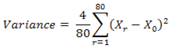
X0 is the estimate calculated using the production weight and Xr is the estimate calculated using the rth replicate weight. The standard error is the square root of the variance. The 90th percent margin of error is 1.645 times the standard error.
For more information on the formation of the replicate weights, see chapter 12 of the Design and Methodology documentation at http://www.census.gov/acs/www/Downloads/survey_methodology/acs_design_methodology_ch12_2014.pdf.
Beginning with the ACS 2011 1-year estimates, a new imputation-based methodology was incorporated into processing (see the description in the Group Quarters Person Weighting Section). An adjustment was made to the production replicate weight variance methodology to account for the non-negligible amount of additional variation being introduced by the new technique.5
Excluding the base weights, replicate weights were allowed to be negative in order to avoid underestimating the standard error. Exceptions include:
1. The estimate of the number or proportion of people, households, families, or housing units in a geographic area with a specific characteristic is zero. A special procedure is used to estimate the standard error.
2. There are either no sample observations available to compute an estimate or standard error of a median, an aggregate, a proportion, or some other ratio, or there are too few sample observations to compute a stable estimate of the standard error. The estimate is represented in the tables by "-" and the margin of error by "**" (two asterisks).
3. The estimate of a median falls in the lower open-ended interval or upper open-ended interval of a distribution. If the median occurs in the lowest interval, then a "-" follows the estimate, and if the median occurs in the upper interval, then a "+" follows the estimate. In both cases the margin of error is represented in the tables by "***" (three asterisks).
5For more information regarding this issue, see Asiala, M. and Castro, E. 2012. Developing Replicate Weight- Based Methods to Account for Imputation Variance in a Mass Imputation Application. In JSM proceedings, Section on Survey Research Methods, Alexandria, VA: American Statistical Association.
The formula provided below calculates the variance using the ACS estimate (X0) and the 80 replicate estimates (Xr).
X0 is the estimate calculated using the production weight and Xr is the estimate calculated using the rth replicate weight. The standard error is the square root of the variance. The 90th percent margin of error is 1.645 times the standard error.
For more information on the formation of the replicate weights, see chapter 12 of the Design and Methodology documentation at http://www.census.gov/acs/www/Downloads/survey_methodology/acs_design_methodology_ch12_2014.pdf.
Beginning with the ACS 2011 1-year estimates, a new imputation-based methodology was incorporated into processing (see the description in the Group Quarters Person Weighting Section). An adjustment was made to the production replicate weight variance methodology to account for the non-negligible amount of additional variation being introduced by the new technique.5
Excluding the base weights, replicate weights were allowed to be negative in order to avoid underestimating the standard error. Exceptions include:
1. The estimate of the number or proportion of people, households, families, or housing units in a geographic area with a specific characteristic is zero. A special procedure is used to estimate the standard error.
2. There are either no sample observations available to compute an estimate or standard error of a median, an aggregate, a proportion, or some other ratio, or there are too few sample observations to compute a stable estimate of the standard error. The estimate is represented in the tables by "-" and the margin of error by "**" (two asterisks).
3. The estimate of a median falls in the lower open-ended interval or upper open-ended interval of a distribution. If the median occurs in the lowest interval, then a "-" follows the estimate, and if the median occurs in the upper interval, then a "+" follows the estimate. In both cases the margin of error is represented in the tables by "***" (three asterisks).
5For more information regarding this issue, see Asiala, M. and Castro, E. 2012. Developing Replicate Weight- Based Methods to Account for Imputation Variance in a Mass Imputation Application. In JSM proceedings, Section on Survey Research Methods, Alexandria, VA: American Statistical Association.
The standard errors estimated from these tables are for individual estimates. Additional calculations are required to estimate the standard errors for sums of or the differences between two or more sample estimates.
The standard error of the sum of two sample estimates is the square root of the sum of the two individual standard errors squared plus a covariance term. That is, for standard errors and
and of estimates
 and
and 

The covariance measures the interactions between two estimates. Currently the covariance terms are not available. Data users should use the approximation:
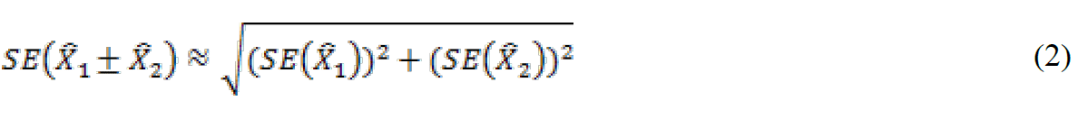
However, this method will underestimate or overestimate the standard error if the two estimates interact in either a positive or negative way.
The approximation formula (2) can be expanded to more than two estimates by adding in the individual standard errors squared inside the radical. As the number of estimates involved in the sum or difference increases, the results of formula (2) become increasingly different from the standard error derived directly from the ACS microdata. Care should be taken to work with the fewest number of estimates as possible. If there are estimates involved in the sum that are controlled in the weighting then the approximate standard error can be increasingly different. Several examples are provided starting on page 32 to demonstrate issues associated with approximating the standard errors when summing large numbers of estimates together.
The standard error of the sum of two sample estimates is the square root of the sum of the two individual standard errors squared plus a covariance term. That is, for standard errors
and of estimates and The covariance measures the interactions between two estimates. Currently the covariance terms are not available. Data users should use the approximation:
However, this method will underestimate or overestimate the standard error if the two estimates interact in either a positive or negative way.
The approximation formula (2) can be expanded to more than two estimates by adding in the individual standard errors squared inside the radical. As the number of estimates involved in the sum or difference increases, the results of formula (2) become increasingly different from the standard error derived directly from the ACS microdata. Care should be taken to work with the fewest number of estimates as possible. If there are estimates involved in the sum that are controlled in the weighting then the approximate standard error can be increasingly different. Several examples are provided starting on page 32 to demonstrate issues associated with approximating the standard errors when summing large numbers of estimates together.
The statistic of interest may be the ratio of two estimates. First is the case where the numerator is not a subset of the denominator. The standard error of this ratio between two sample estimates is approximated as:
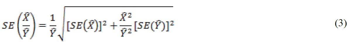
For a proportion (or percent), a ratio where the numerator is a subset of the denominator, a slightly different estimator is used. If  , then the standard error of this proportion is approximated as:
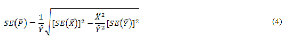
If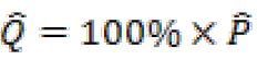 (P is the proportion and Q is its corresponding percent), then
 . Note the difference between the formulas to approximate the standard error for proportions (4) and ratios (3) - the plus sign in the previous formula has been replaced with a minus sign. If the value under the radical is negative, use the ratio standard error formula above, instead.
, then the standard error of this proportion is approximated as:If
(P is the proportion and Q is its corresponding percent), then. Note the difference between the formulas to approximate the standard error for proportions (4) and ratios (3) - the plus sign in the previous formula has been replaced with a minus sign. If the value under the radical is negative, use the ratio standard error formula above, instead.This calculates the percent change from one time period to another, for example, computing the percent change of a 2013 estimate to a 2012 estimate. Normally, the current estimate is compared to the older estimate.
Let the current estimate and the earlier estimate
  then the formula for percent change is:

This reduces to a ratio. The ratio formula above may be used to calculate the standard error. As a caveat, this formula does not take into account the correlation when calculating overlapping time periods.
Let the current estimate
and the earlier estimate then the formula for percent change is:This reduces to a ratio. The ratio formula above may be used to calculate the standard error. As a caveat, this formula does not take into account the correlation when calculating overlapping time periods.
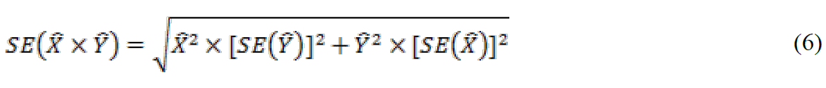
Significant differences - Users may conduct a statistical test to see if the difference between a PRCS estimate and any other chosen estimates is statistically significant at a given confidence level. "Statistically significant" means that the difference is not likely due to random chance alone. With the two estimates (Est1 and Est2) and their respective standard errors (SE1 and SE2), calculate a Z statistic:
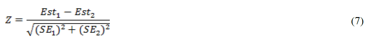
If Z > 1.645 or Z < -1.645, then the difference can be said to be statistically significant at the 90 percent confidence level. 6
Users are also cautioned to not rely on looking at whether confidence intervals for two estimates overlap or not to determine statistical significance, because there are circumstances where that method will not give the correct test result. If two confidence intervals do not overlap, then the estimates will be significantly different (i.e. the significance test will always agree). However, if two confidence intervals do overlap, then the estimates may or may not be significantly different. The Z calculation above is recommended in all cases.
Here is a simple example of why it is not recommended to use the overlapping confidence bounds rule of thumb as a substitute for a statistical test.
Let: X1 = 6.0 with SE1 = 0.5 and X2 = 5.0 with SE2 = 0.2.
The Lower Bound for X1 = 6.0 - 0.5 x 1.645 = 5.2 while the Upper Bound for X2 = 5.0 + 0.2 x 1.645 = 5.3. The confidence bounds overlap, so, the rule of thumb would indicate that the estimates are not significantly different at the 90% level.
However, if we apply the statistical significance test we obtain:
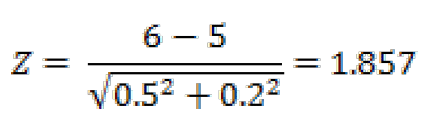
Z = 1.857 > 1.645 which means that the difference is significant (at the 90% level).
All statistical testing in ACS data products is based on the 90 percent confidence level. Users should understand that all testing was done using unrounded estimates and standard errors, and it may not be possible to replicate test results using the rounded estimates and margins of error as published.
6The ACS Accuracy of the Data document in 2005 used a Z statistic of +/-1.65. Data users should use +/-1.65 for estimates published in 2005 or earlier.
If Z > 1.645 or Z < -1.645, then the difference can be said to be statistically significant at the 90 percent confidence level. 6
Users are also cautioned to not rely on looking at whether confidence intervals for two estimates overlap or not to determine statistical significance, because there are circumstances where that method will not give the correct test result. If two confidence intervals do not overlap, then the estimates will be significantly different (i.e. the significance test will always agree). However, if two confidence intervals do overlap, then the estimates may or may not be significantly different. The Z calculation above is recommended in all cases.
Here is a simple example of why it is not recommended to use the overlapping confidence bounds rule of thumb as a substitute for a statistical test.
Let: X1 = 6.0 with SE1 = 0.5 and X2 = 5.0 with SE2 = 0.2.
The Lower Bound for X1 = 6.0 - 0.5 x 1.645 = 5.2 while the Upper Bound for X2 = 5.0 + 0.2 x 1.645 = 5.3. The confidence bounds overlap, so, the rule of thumb would indicate that the estimates are not significantly different at the 90% level.
However, if we apply the statistical significance test we obtain:
Z = 1.857 > 1.645 which means that the difference is significant (at the 90% level).
All statistical testing in ACS data products is based on the 90 percent confidence level. Users should understand that all testing was done using unrounded estimates and standard errors, and it may not be possible to replicate test results using the rounded estimates and margins of error as published.
6The ACS Accuracy of the Data document in 2005 used a Z statistic of +/-1.65. Data users should use +/-1.65 for estimates published in 2005 or earlier.
We will present some examples based on the real data to demonstrate the use of the formulas.
The estimated number of males, never married is 45,175,265 from summary table B12001 for the United States for 2013. The margin of error is 87,709.
Calculating the standard error using the margin of error, we have:

Calculating the standard error using the margin of error, we have:
We are interested in the number of people who have never been married. From Example 1, we know the number of males, never married is 45,175,265. From summary table B12001 we have the number of females, never married is 39,145,401 with a margin of error of 81,710. So, the estimated number of people who have never been married is 45,175,265 + 39,145,401 = 84,320,666. To calculate the approximate standard error of this sum, we need the standard errors of the two estimates in the sum. We have the standard error for the number of males never married from example 1 as 53,319. The standard error for the number of females never married is calculated using the margin of error:

So using formula (2) for the approximate standard error of a sum or difference we have:

Caution: This method will underestimate or overestimate the standard error if the two estimates interact in either a positive or negative way.
To calculate the lower and upper bounds of the 90 percent confidence interval around 84,320,666 using the standard error, simply multiply 72,871 by 1.645, then add and subtract the product from 84,320,666. Thus the 90 percent confidence interval for this estimate is [84,320,666 - 1.645(72,871)] to [84,320,666 + 1.645(72,871)] or 84,200,793 to 84,440,539.
So using formula (2) for the approximate standard error of a sum or difference we have:
Caution: This method will underestimate or overestimate the standard error if the two estimates interact in either a positive or negative way.
To calculate the lower and upper bounds of the 90 percent confidence interval around 84,320,666 using the standard error, simply multiply 72,871 by 1.645, then add and subtract the product from 84,320,666. Thus the 90 percent confidence interval for this estimate is [84,320,666 - 1.645(72,871)] to [84,320,666 + 1.645(72,871)] or 84,200,793 to 84,440,539.
We are interested in the percentage of females who have never been married to the number of people who have never been married. The number of females, never married is 39,145,401 and the number of people who have never been married is 84,320,666. To calculate the approximate standard error of this percent, we need the standard errors of the two estimates in the percent. We have the approximate standard error for the number of females never married from example 2 as 49,672 and the approximate standard error for the number of people never married calculated from example 2 as 72,871.
The estimate is
So, using formula (4) for the approximate standard error of a proportion or percent, we have:

To calculate the lower and upper bounds of the 90 percent confidence interval around 46.42 using the standard error, simply multiply 0.04 by 1.645, then add and subtract the product from 46.42. Thus the 90 percent confidence interval for this estimate is [46.42 - 1.645(0.04)] to [46.42 + 1.645(0.04)], or 46.35 to 46.49.
The estimate is
So, using formula (4) for the approximate standard error of a proportion or percent, we have:
To calculate the lower and upper bounds of the 90 percent confidence interval around 46.42 using the standard error, simply multiply 0.04 by 1.645, then add and subtract the product from 46.42. Thus the 90 percent confidence interval for this estimate is [46.42 - 1.645(0.04)] to [46.42 + 1.645(0.04)], or 46.35 to 46.49.
Now, let us calculate the estimate of the ratio of the number of unmarried males to the number of unmarried females and its approximate standard error. From the above examples, the estimate for the number of unmarried men is 45,175,265 with a standard error of 53,319, and the estimate for the number of unmarried women is 39,145,401 with a standard error of 49,672.
The estimate of the ratio is 45,175,265 / 39,145,401 = 1.154.
Using formula (3) for the approximate standard error of this ratio we have:

The 90 percent margin of error for this estimate would be 0.002 multiplied by 1.645, or about 0.003. The 90 percent lower and upper 90 percent confidence bounds would then be [1.154 – 1.645(0.002)] to [1.154 + 1.645(0.002)], or 1.151 and 1.157.
The estimate of the ratio is 45,175,265 / 39,145,401 = 1.154.
Using formula (3) for the approximate standard error of this ratio we have:
The 90 percent margin of error for this estimate would be 0.002 multiplied by 1.645, or about 0.003. The 90 percent lower and upper 90 percent confidence bounds would then be [1.154 – 1.645(0.002)] to [1.154 + 1.645(0.002)], or 1.151 and 1.157.
We are interested in the number of single unit detached owner-occupied housing units. The number of owner-occupied housing units is 73,843,861 with a margin of error of 212,871 from subject table S2504 for 2013, and the percent of single unit detached owner-occupied housing units is 82.3% (0.823) with a margin of error of 0.1 (0.001). So the number of 1-unit detached owner-occupied housing units is 73,843,861 * 0.823 = 60,773,498. Calculating the standard error for the estimates using the margin of error we have::

and

The approximate standard error for number of 1-unit detached owner-occupied housing units is calculated using formula (5) for products as:

To calculate the lower and upper bounds of the 90 percent confidence interval around 60,773,498 using the standard error, simply multiply 115,574 by 1.645, then add and subtract the product from 60,773,498. Thus the 90 percent confidence interval for this estimate is [60,773,498 - 1.645(115,574)] to [60,773,498 + 1.645(115,574)] or 60,583,379 to 60,963,617.
and
The approximate standard error for number of 1-unit detached owner-occupied housing units is calculated using formula (5) for products as:
To calculate the lower and upper bounds of the 90 percent confidence interval around 60,773,498 using the standard error, simply multiply 115,574 by 1.645, then add and subtract the product from 60,773,498. Thus the 90 percent confidence interval for this estimate is [60,773,498 - 1.645(115,574)] to [60,773,498 + 1.645(115,574)] or 60,583,379 to 60,963,617.
As mentioned earlier, sample data are subject to nonsampling error. This component of error could introduce serious bias into the data, and the total error could increase dramatically over that which would result purely from sampling. While it is impossible to completely eliminate nonsampling error from a survey operation, the Census Bureau attempts to control the sources of such error during the collection and processing operations. Described below are the primary sources of nonsampling error and the programs instituted for control of this error. The success of these programs, however, is contingent upon how well the instructions were carried out during the survey.
A major way to avoid coverage error in a survey is to ensure that its sampling frame, for ACS an address list in each state, is as complete and accurate as possible. The source of addresses for the ACS is the MAF. An attempt is made to assign all appropriate geographic codes to each MAF address via an automated procedure using the Census Bureau TIGER (Topologically Integrated Geographic Encoding and Referencing) files. A manual coding operation based in the appropriate regional offices is attempted for addresses which could not be automatically coded. The MAF was used as the source of addresses for selecting sample housing units and mailing questionnaires. TIGER produced the location maps for CAPI assignments. Sometimes the MAF has an address that is the duplicate of another address already on the MAF. This could occur when there is a slight difference in the address such as 123 Main Street versus 123 Maine Street.
In the CATI and CAPI nonresponse follow-up phases, efforts were made to minimize the chances that housing units that were not part of the sample were interviewed in place of units in sample by mistake. If a CATI interviewer called a mail nonresponse case and was not able to reach the exact address, no interview was conducted and the case was eligible for CAPI. During CAPI follow-up, the interviewer had to locate the exact address for each sample housing unit. If the interviewer could not locate the exact sample unit in a multi-unit structure, or found a different number of units than expected, the interviewers were instructed to list the units in the building and follow a specific procedure to select a replacement sample unit. Person overcoverage can occur when an individual is included as a member of a housing unit but does not meet ACS residency rules.
Coverage rates give a measure of undercoverage or overcoverage of persons or housing units in a given geographic area. Rates below 100 percent indicate undercoverage, while rates above 100 percent indicate overcoverage. Coverage rates are released concurrent with the release of estimates on American FactFinder in the B98 series of detailed tables. Further information about ACS coverage rates may be found at http://www.census.gov/acs/www/methodology/methodology_main/.
- Unit Nonresponse - Unit nonresponse is the failure to obtain data from housing units in the sample. Unit nonresponse may occur because households are unwilling or unable to participate, or because an interviewer is unable to make contact with a housing unit. Unit nonresponse is problematic when there are systematic or variable differences between interviewed and noninterviewed housing units on the characteristics measured by the survey. Nonresponse bias is introduced into an estimate when differences are systematic, while nonresponse error for an estimate evolves from variable differences between interviewed and noninterviewed households.
The ACS makes every effort to minimize unit nonresponse, and thus, the potential for nonresponse error. First, the ACS used a combination of mail, CATI, and CAPI data collection modes to maximize response. The mail phase included a series of three to four mailings to encourage housing units to return the questionnaire. Subsequently, mail nonrespondents (for which phone numbers are available) were contacted by CATI for an interview. Finally, a subsample of the mail and telephone nonrespondents was contacted by personal visit to attempt an interview. Combined, these three efforts resulted in a very high overall response rate for the ACS.
ACS response rates measure the percent of units with a completed interview. The higher the response rate, and consequently the lower the nonresponse rate, the less chance estimates may be affected by nonresponse bias. Response and nonresponse rates, as well as rates for specific types of nonresponse, are released concurrent with the release of estimates on American FactFinder in the B98 series of detailed tables. Further information about response and nonresponse rates may be found at http://www.census.gov/acs/www/methodology/methodology_main/.
- Item Nonresponse - Nonresponse to particular questions on the survey questionnaire and instrument allows for the introduction of error or bias into the data, since the characteristics of the nonrespondents have not been observed and may differ from those reported by respondents. As a result, any imputation procedure using respondent data may not completely reflect this difference either at the elemental level (individual person or housing unit) or on average.
Some protection against the introduction of large errors or biases is afforded by minimizing nonresponse. In the ACS, item nonresponse for the CATI and CAPI operations was minimized by the requirement that the automated instrument receive a response to each question before the next one could be asked. Questionnaires returned by mail were edited for completeness and acceptability. They were reviewed by computer for content omissions and population coverage. If necessary, a telephone follow-up was made to obtain missing information. Potential coverage errors were included in this follow-up.
Allocation tables provide the weighted estimate of persons or housing units for which a value was imputed, as well as the total estimate of persons or housing units that were eligible to answer the question. The smaller the number of imputed responses, the lower the chance that the item nonresponse is contributing a bias to the estimates. Allocation tables are released concurrent with the release of estimates on American Factfinder in the B99 series of detailed tables with the overall allocation rates across all person and housing unit characteristics in the B98 series of detailed tables. Additional information on item nonresponse and allocations can be found at http://www.census.gov/acs/www/methodology/methodology_main/.
- Interviewer monitoring - The interviewer may misinterpret or otherwise incorrectly enter information given by a respondent; may fail to collect some of the information for a person or household; or may collect data for households that were not designated as part of the sample. To control these problems, the work of interviewers was monitored carefully. Field staff were prepared for their tasks by using specially developed training packages that included hands-on experience in using survey materials. A sample of the households interviewed by CAPI interviewers was reinterviewed to control for the possibility that interviewers may have fabricated data.
- Processing Error - The many phases involved in processing the survey data represent potential sources for the introduction of nonsampling error. The processing of the survey questionnaires includes the keying of data from completed questionnaires, automated clerical review, follow-up by telephone, manual coding of write-in responses, and automated data processing. The various field, coding and computer operations undergo a number of quality control checks to insure their accurate application.
- Content Editing - After data collection was completed, any remaining incomplete or inconsistent information was imputed during the final content edit of the collected data. Imputations, or computer assignments of acceptable codes in place of unacceptable entries or blanks, were needed most often when an entry for a given item was missing or when the information reported for a person or housing unit on that item was inconsistent with other information for that same person or housing unit. As in other surveys and previous censuses, the general procedure for changing unacceptable entries was to allocate an entry for a person or housing unit that was consistent with entries for persons or housing units with similar characteristics. Imputing acceptable values in place of blanks or unacceptable entries enhances the usefulness of the data.
- Coverage Error
A major way to avoid coverage error in a survey is to ensure that its sampling frame, for ACS an address list in each state, is as complete and accurate as possible. The source of addresses for the ACS is the MAF. An attempt is made to assign all appropriate geographic codes to each MAF address via an automated procedure using the Census Bureau TIGER (Topologically Integrated Geographic Encoding and Referencing) files. A manual coding operation based in the appropriate regional offices is attempted for addresses which could not be automatically coded. The MAF was used as the source of addresses for selecting sample housing units and mailing questionnaires. TIGER produced the location maps for CAPI assignments. Sometimes the MAF has an address that is the duplicate of another address already on the MAF. This could occur when there is a slight difference in the address such as 123 Main Street versus 123 Maine Street.
In the CATI and CAPI nonresponse follow-up phases, efforts were made to minimize the chances that housing units that were not part of the sample were interviewed in place of units in sample by mistake. If a CATI interviewer called a mail nonresponse case and was not able to reach the exact address, no interview was conducted and the case was eligible for CAPI. During CAPI follow-up, the interviewer had to locate the exact address for each sample housing unit. If the interviewer could not locate the exact sample unit in a multi-unit structure, or found a different number of units than expected, the interviewers were instructed to list the units in the building and follow a specific procedure to select a replacement sample unit. Person overcoverage can occur when an individual is included as a member of a housing unit but does not meet ACS residency rules.
Coverage rates give a measure of undercoverage or overcoverage of persons or housing units in a given geographic area. Rates below 100 percent indicate undercoverage, while rates above 100 percent indicate overcoverage. Coverage rates are released concurrent with the release of estimates on American FactFinder in the B98 series of detailed tables. Further information about ACS coverage rates may be found at http://www.census.gov/acs/www/methodology/methodology_main/.
- Nonresponse Error
- Unit Nonresponse - Unit nonresponse is the failure to obtain data from housing units in the sample. Unit nonresponse may occur because households are unwilling or unable to participate, or because an interviewer is unable to make contact with a housing unit. Unit nonresponse is problematic when there are systematic or variable differences between interviewed and noninterviewed housing units on the characteristics measured by the survey. Nonresponse bias is introduced into an estimate when differences are systematic, while nonresponse error for an estimate evolves from variable differences between interviewed and noninterviewed households.
The ACS makes every effort to minimize unit nonresponse, and thus, the potential for nonresponse error. First, the ACS used a combination of mail, CATI, and CAPI data collection modes to maximize response. The mail phase included a series of three to four mailings to encourage housing units to return the questionnaire. Subsequently, mail nonrespondents (for which phone numbers are available) were contacted by CATI for an interview. Finally, a subsample of the mail and telephone nonrespondents was contacted by personal visit to attempt an interview. Combined, these three efforts resulted in a very high overall response rate for the ACS.
ACS response rates measure the percent of units with a completed interview. The higher the response rate, and consequently the lower the nonresponse rate, the less chance estimates may be affected by nonresponse bias. Response and nonresponse rates, as well as rates for specific types of nonresponse, are released concurrent with the release of estimates on American FactFinder in the B98 series of detailed tables. Further information about response and nonresponse rates may be found at http://www.census.gov/acs/www/methodology/methodology_main/.
- Item Nonresponse - Nonresponse to particular questions on the survey questionnaire and instrument allows for the introduction of error or bias into the data, since the characteristics of the nonrespondents have not been observed and may differ from those reported by respondents. As a result, any imputation procedure using respondent data may not completely reflect this difference either at the elemental level (individual person or housing unit) or on average.
Some protection against the introduction of large errors or biases is afforded by minimizing nonresponse. In the ACS, item nonresponse for the CATI and CAPI operations was minimized by the requirement that the automated instrument receive a response to each question before the next one could be asked. Questionnaires returned by mail were edited for completeness and acceptability. They were reviewed by computer for content omissions and population coverage. If necessary, a telephone follow-up was made to obtain missing information. Potential coverage errors were included in this follow-up.
Allocation tables provide the weighted estimate of persons or housing units for which a value was imputed, as well as the total estimate of persons or housing units that were eligible to answer the question. The smaller the number of imputed responses, the lower the chance that the item nonresponse is contributing a bias to the estimates. Allocation tables are released concurrent with the release of estimates on American Factfinder in the B99 series of detailed tables with the overall allocation rates across all person and housing unit characteristics in the B98 series of detailed tables. Additional information on item nonresponse and allocations can be found at http://www.census.gov/acs/www/methodology/methodology_main/.
- Measurement and Processing Error
- Interviewer monitoring - The interviewer may misinterpret or otherwise incorrectly enter information given by a respondent; may fail to collect some of the information for a person or household; or may collect data for households that were not designated as part of the sample. To control these problems, the work of interviewers was monitored carefully. Field staff were prepared for their tasks by using specially developed training packages that included hands-on experience in using survey materials. A sample of the households interviewed by CAPI interviewers was reinterviewed to control for the possibility that interviewers may have fabricated data.
- Processing Error - The many phases involved in processing the survey data represent potential sources for the introduction of nonsampling error. The processing of the survey questionnaires includes the keying of data from completed questionnaires, automated clerical review, follow-up by telephone, manual coding of write-in responses, and automated data processing. The various field, coding and computer operations undergo a number of quality control checks to insure their accurate application.
- Content Editing - After data collection was completed, any remaining incomplete or inconsistent information was imputed during the final content edit of the collected data. Imputations, or computer assignments of acceptable codes in place of unacceptable entries or blanks, were needed most often when an entry for a given item was missing or when the information reported for a person or housing unit on that item was inconsistent with other information for that same person or housing unit. As in other surveys and previous censuses, the general procedure for changing unacceptable entries was to allocate an entry for a person or housing unit that was consistent with entries for persons or housing units with similar characteristics. Imputing acceptable values in place of blanks or unacceptable entries enhances the usefulness of the data.
Several examples are provided here to demonstrate how different the approximated standard errors of sums can be compared to those derived and published with ACS microdata.
A. Suppose we wish to estimate the total number of males with income below the poverty level in the past 12 months using both state and PUMA level estimates for the state of Wyoming. Part of the collapsed table C17001 is displayed below with estimates and their margins of error in parentheses.
Table A: 2009 Estimates of Males with Income Below Poverty from table C17001: Poverty Status in the Past 12 Months by Sex by Age
The first way is to sum the three age groups for Wyoming:
Estimate(Male) = 8,479 + 12,976 + 1,546 = 23,001.
The first approximation for the standard error in this case gives us:
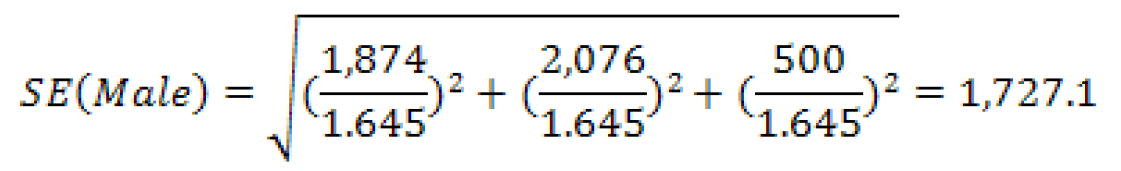
A second way is to sum the four PUMA estimates for Male to obtain:
Estimate(Male) = 5,264 + 6,508 + 4,364 + 6,865 = 23,001 as before.
The second approximation for the standard error yields:
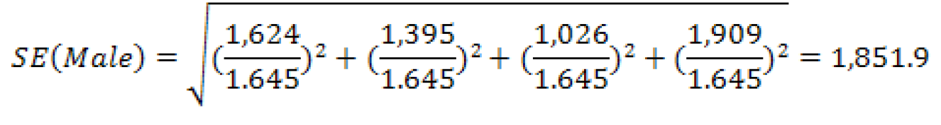
Finally, we can sum up all three age groups for all four PUMAs to obtain an estimate based on a total of twelve estimates:

And the third approximated standard error is
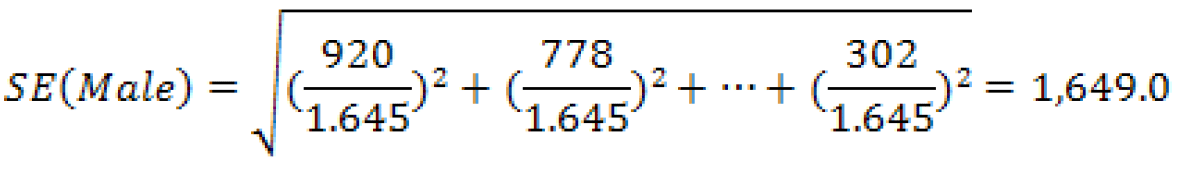
However, we do know that the standard error using the published MOE is 3,309 /1.645 = 2,011.6. In this instance, all of the approximations under-estimate the published standard error and should be used with caution.
B. Suppose we wish to estimate the total number of males at the national level using age and citizenship status. The relevant data from table B05003 is displayed in table B below.
Table B: 2009 Estimates of males from B05003: Sex by Age by Citizenship Status
The estimate and its MOE are actually published. However, if they were not available in the tables, one way of obtaining them would be to add together the number of males under 18 and over 18 to get:

And the first approximated standard error is
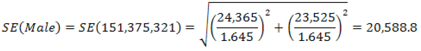
Another way would be to add up the estimates for the three subcategories (Native, and the two subcategories for Foreign Born: Naturalized U.S. Citizen, and Not a U.S. Citizen), for males under and over 18 years of age. From these six estimates we obtain:
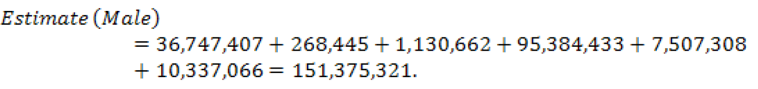
With a second approximated standard error of:
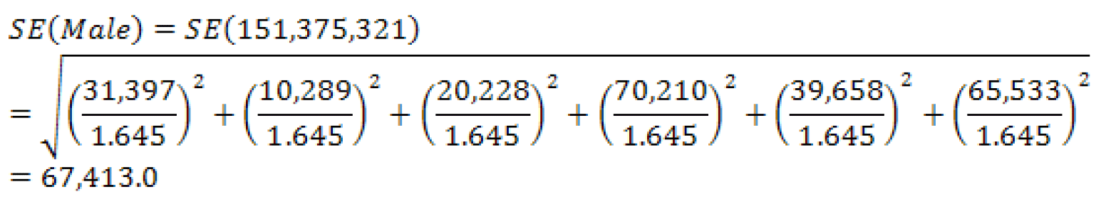
We do know that the standard error using the published margin of error is 27,279 / 1.645 = 16,583.0. With a quick glance, we can see that the ratio of the standard error of the first method to the published-based standard error yields 1.24; an over-estimate of roughly 24%, whereas the second method yields a ratio of 4.07 or an over-estimate of 307%. This is an example of what could happen to the approximate SE when the sum involves a controlled estimate. In this case, it is sex by age.
C. Suppose we are interested in the total number of people aged 65 or older and its standard error. Table C shows some of the estimates for the national level from table B01001 (the estimates in gray were derived for the purpose of this example only).
Table C: Some Estimates from AFF Table B01001: Sex by Age for 2009
To begin we find the total number of people aged 65 and over by simply adding the totals for males and females to get 16,781,175 + 22,725,542 = 39,506,717. One way we could use is summing males and female for each age category and then using their MOEs to approximate the standard error for the total number of people over 65.
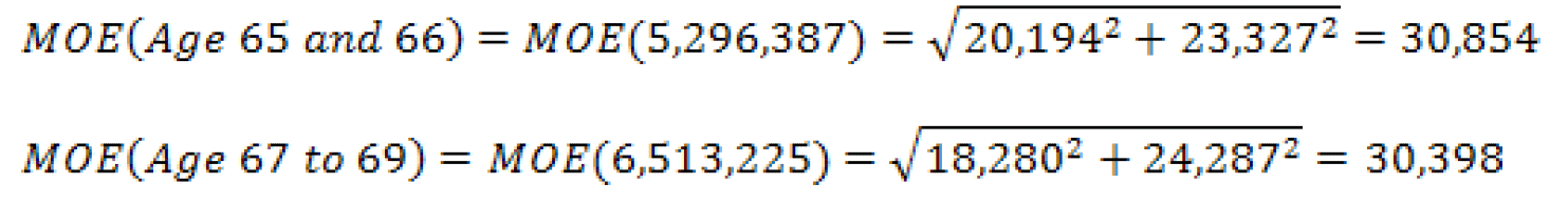
... etc. ...
Now, we calculate for the number of people aged 65 or older to be 39,506,648 using the six derived estimates and approximate the standard error:
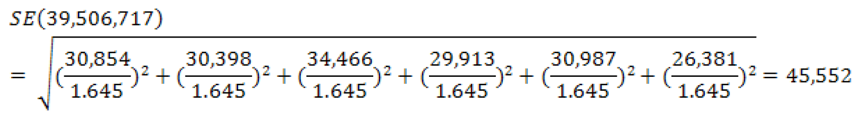
For this example the estimate and its MOE are published in table B09017. The total number of people aged 65 or older is 39,506,648 with a margin of error of 20,689. Therefore the published- based standard error is:
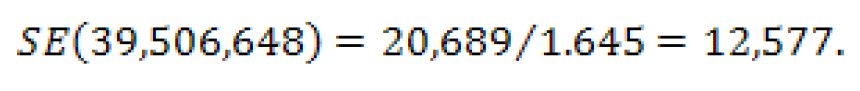
The approximated standard error, using six derived age group estimates, yields an approximated standard error roughly 3.6 times larger than the published-based standard error.
As a note, there are two additional ways to approximate the standard error of people aged 65 and over in addition to the way used above. The first is to find the published MOEs for the males age 65 and older and of females aged 65 and older separately and then combine to find the approximate standard error for the total. The second is to use all twelve of the published estimates together, that is, all estimates from the male age categories and female age categories, to create the SE for people aged 65 and older. However, in this particular example, the results from all three ways are the same. So no matter which way you use, you will obtain the same approximation for the SE. This is different from the results seen in example A.
D. For an alternative to approximating the standard error for people 65 years and older seen in part C, we could find the estimate and its SE by summing all of the estimate for the ages less than 65 years old and subtracting them from the estimate for the total population. Due to the large number of estimates, Table D does not show all of the age groups. In addition, the estimates in part of the table shaded gray were derived for the purposes of this example only and cannot be found in base table B01001.
Table D: Some Estimates from AFF Table B01001: Sex by Age for 2009:
An estimate for the number of people age 65 and older is equal to the total population minus the population between the ages of zero and 64 years old:
Number of people aged 65 and older: 307,006,556 - 267,499,908 = 39,506,648.
The way to approximate the SE is the same as in part C. First we will sum male and female estimates across each age category and then approximate the MOEs. We will use that information to approximate the standard error for our estimate of interest:
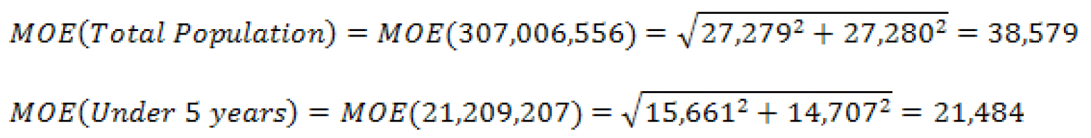
... etc. ...
And the SE for the total number of people aged 65 and older is:
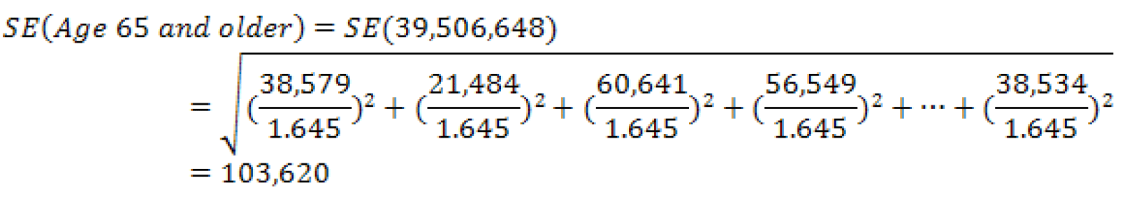
Again, as in Example C, the estimate and its MOE are we published in B09017. The total number of people aged 65 or older is 39,506,648 with a margin of error of 20,689. Therefore the standard error is:

The approximated standard error using the thirteen derived age group estimates yields a standard error roughly 8.2 times larger than the actual SE.
Data users can mitigate the problems shown in examples A through D to some extent by utilizing a collapsed version of a detailed table (if it is available) which will reduce the number of estimates used in the approximation. These issues may also be avoided by creating estimates and SEs using the Public Use Microdata Sample (PUMS) or by requesting a custom tabulation, a fee- based service offered under certain conditions by the Census Bureau. More information regarding custom tabulations may be found at http://www.census.gov/acs/www/data_documentation/custom_tabulations/.
A. Suppose we wish to estimate the total number of males with income below the poverty level in the past 12 months using both state and PUMA level estimates for the state of Wyoming. Part of the collapsed table C17001 is displayed below with estimates and their margins of error in parentheses.
Table A: 2009 Estimates of Males with Income Below Poverty from table C17001: Poverty Status in the Past 12 Months by Sex by Age
| Characteristic | Wyoming | PUMA 00100 | PUMA 00200 | PUMA 00300 | PUMA 00400 |
| Male | 23,001 (3,309) | 5,264 (1,624) | 6,508 (1,395) | 4,364 (1,026) | 6,865 (1,909) |
| Under 18 Years Old | 8,479 (1,874) | 2,041 (920) | 2,222 (778) | 1,999 (750) | 2,217 (1,192) |
| 18 to 64 Years Old | 12,976 (2,076) | 3,004 (1,049) | 3,725 (935) | 2,050 (635) | 4,197 (1,134) |
| 65 Years and Older | 1546 (500) | 219 (237) | 561 (286) | 315 (173) | 451 (302) |
| 2009 American FactFinder | |||||
The first way is to sum the three age groups for Wyoming:
Estimate(Male) = 8,479 + 12,976 + 1,546 = 23,001.
The first approximation for the standard error in this case gives us:
A second way is to sum the four PUMA estimates for Male to obtain:
Estimate(Male) = 5,264 + 6,508 + 4,364 + 6,865 = 23,001 as before.
The second approximation for the standard error yields:
Finally, we can sum up all three age groups for all four PUMAs to obtain an estimate based on a total of twelve estimates:
And the third approximated standard error is
However, we do know that the standard error using the published MOE is 3,309 /1.645 = 2,011.6. In this instance, all of the approximations under-estimate the published standard error and should be used with caution.
B. Suppose we wish to estimate the total number of males at the national level using age and citizenship status. The relevant data from table B05003 is displayed in table B below.
Table B: 2009 Estimates of males from B05003: Sex by Age by Citizenship Status
| Characteristic | Estimate | MOE |
| Male | 151,375,321 | 27,279 |
| Under 18 Years | 38,146,514 | 24,365 |
| Native | 36,747,407 | 31,397 |
| Foreign Born | 1,399,107 | 20,177 |
| Naturalized U.S. Citizen | 268,445 | 10,289 |
| Not a U.S. Citizen | 1,130,662 | 20,228 |
| 18 Years and Older | 113,228,807 | 23,525 |
| Native | 95,384,433 | 70,210 |
| Foreign Born | 17,844,374 | 59,750 |
| Naturalized U.S. Citizen | 7,507,308 | 39,658 |
| Not a U.S. Citizen | 10,337,066 | 65,533 |
| 2009 American FactFinder | ||
The estimate and its MOE are actually published. However, if they were not available in the tables, one way of obtaining them would be to add together the number of males under 18 and over 18 to get:
And the first approximated standard error is
Another way would be to add up the estimates for the three subcategories (Native, and the two subcategories for Foreign Born: Naturalized U.S. Citizen, and Not a U.S. Citizen), for males under and over 18 years of age. From these six estimates we obtain:
With a second approximated standard error of:
We do know that the standard error using the published margin of error is 27,279 / 1.645 = 16,583.0. With a quick glance, we can see that the ratio of the standard error of the first method to the published-based standard error yields 1.24; an over-estimate of roughly 24%, whereas the second method yields a ratio of 4.07 or an over-estimate of 307%. This is an example of what could happen to the approximate SE when the sum involves a controlled estimate. In this case, it is sex by age.
C. Suppose we are interested in the total number of people aged 65 or older and its standard error. Table C shows some of the estimates for the national level from table B01001 (the estimates in gray were derived for the purpose of this example only).
Table C: Some Estimates from AFF Table B01001: Sex by Age for 2009
| Age Category | Estimate, Male | MOE, Male | Estimate, Female | MOE, Female | Total | Estimated MOE, Total |
| 65 and 66 years old | 2,492,871 | 20,194 | 2,803,516 | 23,327 | 5,296,387 | 30,854 |
| 67 to 69 years old | 3,029,709 | 18,280 | 3,483,447 | 24,287 | 6,513,225 | 30,398 |
| 70 to 74 years old | 4,088,428 | 21,588 | 4,927,666 | 26,867 | 9,016,094 | 34,466 |
| 75 to 79 years old | 3,168,175 | 19,097 | 4,204,401 | 23,024 | 7,372,576 | 29,913 |
| 80 to 84 years old | 2,258,021 | 17,716 | 3,538,869 | 25,423 | 5,796,890 | 30,987 |
| 85 years and older | 1,743,971 | 17,991 | 3,767,574 | 19,294 | 5,511,545 | 26,381 |
| Total | 16,781,175 | NA | 22,725,473 | NA | 39,506,648 | 74,932 |
| 2009 American FactFinder | ||||||
To begin we find the total number of people aged 65 and over by simply adding the totals for males and females to get 16,781,175 + 22,725,542 = 39,506,717. One way we could use is summing males and female for each age category and then using their MOEs to approximate the standard error for the total number of people over 65.
... etc. ...
Now, we calculate for the number of people aged 65 or older to be 39,506,648 using the six derived estimates and approximate the standard error:
For this example the estimate and its MOE are published in table B09017. The total number of people aged 65 or older is 39,506,648 with a margin of error of 20,689. Therefore the published- based standard error is:
The approximated standard error, using six derived age group estimates, yields an approximated standard error roughly 3.6 times larger than the published-based standard error.
As a note, there are two additional ways to approximate the standard error of people aged 65 and over in addition to the way used above. The first is to find the published MOEs for the males age 65 and older and of females aged 65 and older separately and then combine to find the approximate standard error for the total. The second is to use all twelve of the published estimates together, that is, all estimates from the male age categories and female age categories, to create the SE for people aged 65 and older. However, in this particular example, the results from all three ways are the same. So no matter which way you use, you will obtain the same approximation for the SE. This is different from the results seen in example A.
D. For an alternative to approximating the standard error for people 65 years and older seen in part C, we could find the estimate and its SE by summing all of the estimate for the ages less than 65 years old and subtracting them from the estimate for the total population. Due to the large number of estimates, Table D does not show all of the age groups. In addition, the estimates in part of the table shaded gray were derived for the purposes of this example only and cannot be found in base table B01001.
Table D: Some Estimates from AFF Table B01001: Sex by Age for 2009:
| Age Category | Estimate, Male | MOE, Male | Estimate, Female | MOE, Female | Total | Estimated MOE, Total |
| Total Population | 151,375,321 | 27,279 | 155,631,235 | 27,280 | 307,006,556 | 38,579 |
| Under 5 years | 10,853,263 | 15,661 | 10,355,944 | 14,707 | 21,209,207 | 21,484 |
| 5 to 9 years old | 10,273,948 | 43,555 | 9,850,065 | 42,194 | 20,124,013 | 60,641 |
| 10 to 14 years old | 10,532,166 | 40,051 | 9,985,327 | 39,921 | 20,517,493 | 56,549 |
| ... | ... | ... | ... | ... | ||
| 62 to 64 years old | 4,282,178 | 25,636 | 4,669,376 | 28,769 | 8,951,554 | 38,534 |
| Total for Age 0 to 64 years old | 134,594,146 | 117,166 | 132,905,762 | 117,637 | 267,499,908 | 166,031 |
| Total for Age 65 years and older | 16,781,175 | 120,300 | 22,725,473 | 120,758 | 39,506,648 | 170,454 |
| 2009 American FactFinder | ||||||
An estimate for the number of people age 65 and older is equal to the total population minus the population between the ages of zero and 64 years old:
Number of people aged 65 and older: 307,006,556 - 267,499,908 = 39,506,648.
The way to approximate the SE is the same as in part C. First we will sum male and female estimates across each age category and then approximate the MOEs. We will use that information to approximate the standard error for our estimate of interest:
... etc. ...
And the SE for the total number of people aged 65 and older is:
Again, as in Example C, the estimate and its MOE are we published in B09017. The total number of people aged 65 or older is 39,506,648 with a margin of error of 20,689. Therefore the standard error is:
The approximated standard error using the thirteen derived age group estimates yields a standard error roughly 8.2 times larger than the actual SE.
Data users can mitigate the problems shown in examples A through D to some extent by utilizing a collapsed version of a detailed table (if it is available) which will reduce the number of estimates used in the approximation. These issues may also be avoided by creating estimates and SEs using the Public Use Microdata Sample (PUMS) or by requesting a custom tabulation, a fee- based service offered under certain conditions by the Census Bureau. More information regarding custom tabulations may be found at http://www.census.gov/acs/www/data_documentation/custom_tabulations/.
The data contained in these data products are based on the Puerto Rico Community Survey (PRCS) sample interviewed from January 1, 2013 through December 31, 2013. The PRCS sample is selected from all municipios in Puerto Rico (PR). Data for Puerto Rico was first released in 2005. In 2006, the PRCS began collection of data from sampled persons in group quarters (GQs) – for example, military barracks, college dormitories, nursing homes, and correctional facilities. Persons in group quarters are included with persons in housing units (HUs) in all 2013 PRCS estimates that are based on the total population. All PRCS population estimates from years prior to 2006 include only persons in housing units. The PRCS, like any other statistical activity, is subject to error. The purpose of this documentation is to provide data users with a basic understanding of the PRCS sample design, estimation methodology, and accuracy of the PRCS data. The PRCS is sponsored by the U.S. Census Bureau, and is part of the Decennial Census Program.
Additional information on the design and methodology of the PRCS, including data collection and processing, can be found at:
http://www.census.gov/acs/www/methodology/methodology_main/.
The 2013 Accuracy of the Data for the United States can be found at:
http://www.census.gov/acs/www/Downloads/data_documentation/Accuracy/PRCS_Accuracy_of_Data_2013.pdf.
The PRCS employs three modes of data collection:
Month 1: Addresses in sample that are determined to be mailable are sent a questionnaire via the U.S. Postal Service.
Month 2: All mail non-responding addresses with an available phone number are sent to CATI.
Month 3: A sample of mail non-responses without a phone number, CATI non-responses, and unmailable addresses are selected and sent to CAPI.
Note that mail responses are accepted during all three months of data collection.
- Internet
- Mailout/Mailback
- Computer Assisted Telephone Interview (CATI)
- Computer Assisted Personal Interview (CAPI)
Month 1: Addresses in sample that are determined to be mailable are sent a questionnaire via the U.S. Postal Service.
Month 2: All mail non-responding addresses with an available phone number are sent to CATI.
Month 3: A sample of mail non-responses without a phone number, CATI non-responses, and unmailable addresses are selected and sent to CAPI.
Note that mail responses are accepted during all three months of data collection.
Field representatives have several options available to them for data collection. These include completing the questionnaire while speaking to the resident in person or over the telephone, conducting a personal interview with a proxy, such as a relative or guardian, or leaving paper questionnaires for residents to complete for themselves and then pick them up later. This last option is used for data collection in Federal prisons.
Group Quarters data collection spans six weeks, except for Federal prisons, where the data collection time period is four months. All Federal prisons are assigned to September with a four month data collection window.
Group Quarters data collection spans six weeks, except for Federal prisons, where the data collection time period is four months. All Federal prisons are assigned to September with a four month data collection window.
The universe for the PRCS consists of all valid, residential housing unit addresses in all municipios in Puerto Rico. The Master Address File (MAF) is a database maintained by the Census Bureau containing a listing of residential and commercial addresses in the U.S. and Puerto Rico. The MAF is updated twice each year with the Delivery Sequence Files provided by the U.S. Postal Service, however this update covers only the U.S. The DSF does not provide changes and updates to the MAF for Puerto Rico. The MAF is also updated with the results from various Census Bureau field operations, including the PRCS.
As a result of operational difficulties associated with data collection, the PRCS excludes certain types of GQs from the sampling universe and data collection operations. The weighting and estimation account for this segment of the population as the population in these types of GQs is included in the population controls. The following GQ types were removed from the GQ universe:
- Soup kitchens
- Domestic violence shelters
- Regularly scheduled mobile food vans
- Targeted non-sheltered outdoor locations
- Maritime/merchant vessels
- Living quarters for victims of natural disasters
- Dangerous encampments
The PRCS employs a two-phase, two-stage sample design. The PRCS first-phase sample consists of two separate samples, Main and Supplemental, each chosen at different points in time. Together, these constitute the first-phase sample. Both the Main and the Supplemental samples are chosen in two stages referred to as first- and second-stage sampling. Subsequent to second-stage sampling, sample addresses are randomly assigned to one of the twelve months of the sample year. The second-phase of sampling occurs when the CAPI sample is selected (see Section 2 below).
The Main sample is selected during the summer preceding the sample year. Each address in sample is randomly assigned to one of the 12 months of the sample year. Supplemental sampling occurs in January/February of the sample year, however typically there is no supplemental sample selected in Puerto Rico. Supplemental sampling is done in order to capture growth on the MAF as well as updated geography and addresses information that occurs during the year. There are no significant updates to the Puerto Rico MAF between censuses, so the entire Puerto Rico annual sample is selected during main sampling. A sub-sample of non- responding addresses and of any addresses deemed unmailable is selected for the CAPI data collection mode.
Several of the steps used to select the first-phase sample are common to both Main and Supplemental sampling. The descriptions of the steps included in the first-phase sample selection below indicate which are common to both and which are unique to either Main or Supplemental sampling.
1. First-phase Sample Selection
The measure of size is an estimate of the number of occupied HUs in the Municipio. This is calculated by multiplying the number of PRCS addresses by the occupancy rate from the 2010 Census at the block level. A measure of size for each Census Tract is also calculated in the same manner.
Each block is then assigned the smallest measure of size from the set of all entities of which it is a part. The second-stage sampling strata and the overall first-phase sampling rates are shown in Table 1 below.
2. Second-phase Sample Selection - Subsampling the Unmailable and Non-Responding Addresses
All addresses determined to be unmailable are subsampled for the CAPI phase of data collection at a rate of 2-in-3. Unmailable addresses do not go to the CATI phase of data collection. All addresses for which no response has been obtained prior to CAPI are subsampled at a rate of 1-in-2. Puerto Rico CAPI rates are summarized in Table 2.
Table 2. Second-Phase (CAPI) Subsampling Rates for Puerto Rico
The Main sample is selected during the summer preceding the sample year. Each address in sample is randomly assigned to one of the 12 months of the sample year. Supplemental sampling occurs in January/February of the sample year, however typically there is no supplemental sample selected in Puerto Rico. Supplemental sampling is done in order to capture growth on the MAF as well as updated geography and addresses information that occurs during the year. There are no significant updates to the Puerto Rico MAF between censuses, so the entire Puerto Rico annual sample is selected during main sampling. A sub-sample of non- responding addresses and of any addresses deemed unmailable is selected for the CAPI data collection mode.
Several of the steps used to select the first-phase sample are common to both Main and Supplemental sampling. The descriptions of the steps included in the first-phase sample selection below indicate which are common to both and which are unique to either Main or Supplemental sampling.
1. First-phase Sample Selection
- First-stage sampling (performed during both Main and Supplemental sampling) - First stage sampling defines the universe for the second stage of sampling through two steps. First, all addresses that were in a first-phase sample within the past four years are excluded from eligibility. This ensures that no address is in sample more than once in any five-year period. The second step is to select a 20 percent systematic sample of "new" units, i.e. those units that have never appeared on a previous MAF extract. Each new address is systematically assigned to either the current year or to one of four back- samples. This procedure maintains five equal partitions of the universe.
- Assignment of blocks to a second-stage sampling stratum (performed during Main sampling only) - Second-stage sampling uses five sampling strata in PR. The stratum level rates used in second-stage sampling account for the first-stage selection probabilities. These rates are applied at a block level to addresses in PR by calculating a measure of size for Municipios.
The measure of size is an estimate of the number of occupied HUs in the Municipio. This is calculated by multiplying the number of PRCS addresses by the occupancy rate from the 2010 Census at the block level. A measure of size for each Census Tract is also calculated in the same manner.
Each block is then assigned the smallest measure of size from the set of all entities of which it is a part. The second-stage sampling strata and the overall first-phase sampling rates are shown in Table 1 below.
- Calculation of the second-stage sampling rates (performed during Main sampling only) - The overall first-phase sampling rates given in Table 1 are calculated using the distribution of PRCS valid addresses by second-stage sampling stratum in such a way as to yield an overall target sample size for the year of approximately 36,000. The first- phase rates are adjusted for the first-stage sample to yield the second-stage selection probabilities.
- Second-stage sample selection (performed in Main and Supplemental) - After each block is assigned to a second-stage sampling stratum, a systematic sample of addresses is selected from the second-stage universe (first-stage sample) within each municipio.
- Sample Month Assignment (performed in Main and Supplemental) - After the second stage of sampling, all sample addresses are randomly assigned to a sample month. Addresses selected during Main sampling are allocated to each of the 12 months.
| Sampling Stratum | Type of Area | Rate Definitions | 2013 Sampling Rate |
| 1 | 0 < MOS1 ≤ 200 | 15% | 15.00% |
| 2 | 200 < MOS ≤ 400 | 10% | 10.00% |
| 3 | 400 < MOS ≤ 800 | 7% | 7.00% |
| 4 | 800 < MOS ≤ 1,200 | 2.8 × BR | 3.95% |
| 5 | 0 < TRACTMOS2 ≤ 400 | 3.5 × BR | 4.94% |
| 7 | 400 < TRACTMOS ≤ 1,000 | 2.8 × BR | 3.95% |
| 9 | 1,000 < TRACTMOS ≤ 2,000 | 1.7 × BR | 2.40% |
| 11 | 2,000 < TRACTMOS ≤ 4,000 | BR3 | 1.41% |
| 13 | 4,000 < TRACTMOS ≤ 6,000 | 0.6 × BR | 0.85% |
| 15 | 6,000 < TRACTMOS | 0.35 × BR | 0.49% |
| Note: A subset of sampling strata is listed here since not all of the stateside sampling strata are defined in Puerto Rico. | |||
| 1MOS = measure of size (estimated number occupied housing units) of the smallest governmental entity | |||
| 2TRACTMOS = the measure of size (MOS) at the Census Tract level | |||
| 3BR = base sampling rate | |||
2. Second-phase Sample Selection - Subsampling the Unmailable and Non-Responding Addresses
All addresses determined to be unmailable are subsampled for the CAPI phase of data collection at a rate of 2-in-3. Unmailable addresses do not go to the CATI phase of data collection. All addresses for which no response has been obtained prior to CAPI are subsampled at a rate of 1-in-2. Puerto Rico CAPI rates are summarized in Table 2.
Table 2. Second-Phase (CAPI) Subsampling Rates for Puerto Rico
| Address Characteristics | CAPI Subsampling Rate |
| Unmailable addresses | 66.7% |
| Mailable addresses | 50.0% |
The 2013 group quarters (GQ) sampling frame was divided into two strata: a small GQ stratum and a large GQ stratum. Small GQs have expected populations of fifteen or fewer residents, while large GQs have expected populations of more than fifteen residents.
Samples were selected in two phases within each stratum. In general, GQs were selected in the first phase and then persons/residents were selected in the second phase. Both phases differ between the two strata. Each sampled GQ was randomly assigned to one or more months in 2013 - it was in these months that their person samples were selected.
1. Small GQ Stratum
A. First phase of sample selection
There were two stages of selecting small GQs for sample.
i. First stage
The small GQ universe is divided into five groups that are approximately equal in size. All new small GQs are systematically assigned to one of these five groups on a yearly basis, with about the same probability (20 percent) of being assigned to any given group. Each group represents a second-stage sampling frame, from which GQs are selected once every five years. The 2013 second-stage sampling frame was used in 2008 as well, and is currently to be used in 2018, 2023, etc.
ii. Second stage
GQs were systematically selected from the 2013 second-stage sampling frame. Each GQ had the same second-stage probability of being selected.
B. Second phase of sample selection
Persons were selected for sample from each GQ that was selected for sample in the first phase of sample selection. If fifteen or fewer persons were residing at a GQ at the time a field representative (interviewer) visited the GQ, then all persons were selected for sample. Otherwise, if more than fifteen persons were residing at the GQ, then the interviewer selected a systematic sample of ten persons from the GQ's roster.
C. Targeted sampling rate (probability of selection)
The probability of selecting any given person in a small GQ reflects both phases of sample selection, which was 2.33 percent in Puerto Rico. The sample was designed to have a one-hundred percent sampling rate in the second phase, however, given the expected population for each small GQ (fifteen or fewer persons). This means the probability of selecting any person in a small GQ is also the probability of selecting the small GQ itself. This probability is also the "targeted" sampling rate, as it is this rate around which the sample design is based.
2. Large GQ Stratum
A. First phase of sample selection
All large GQs were eligible for being sampled in 2013, as has been the case every year since the GQ sample's inception in 2006. This means there was only a single stage of sampling in this phase. This stage consists of systematically assigning "hits" to GQs, where each hit represents ten persons to be sampled.
In general, a GQ has either Z or Z+1 hits assigned to it. The value for Z is dependent on both the GQ's expected population size and its targeted sampling rate (section 2.C. below). When this rate is multiplied by a GQ's expected population, the result is a GQ's expected person sample size. If a GQ's expected person sample size is less than ten, then Z = 0; if it is at least ten but less than twenty, then Z = 1; if it is at least twenty but less than thirty, then Z = 2; and so on. See 2.C. below for a detailed example.
If a GQ has an expected person sample size that is less than ten, then this method effectively gives the GQ a probability of selection that is proportional to its size; this probability is the expected person sample size divided by ten. If a GQ has an expected person sample size of ten or more, then it is in sample with certainty and is assigned one or more hits.
B. Second phase of sample selection
Persons were selected within each GQ to which one or more hits were assigned in the first phase of selection. There were ten persons selected at a GQ for every hit assigned to the GQ. The persons were systematically sampled from a roster of persons residing at the GQ at the time of an interviewer's visit. The exception was if there were far fewer persons residing in a GQ than expected - in these situations, the number of persons to sample at the GQ would be reduced to reflect the GQ's actual population. In cases where fewer than ten persons resided in a GQ at the time of a visit, the interviewer would select all of the persons for sample.
C. Targeted sampling rate (probability of selection)
The probability of selecting any given person in a large GQ reflects both phases of sample selection, which was 2.33 percent in Puerto Rico (same as for small GQs). This probability is also the "targeted" sampling rate, as it is this rate around which the sample design is based.
For example, suppose a GQ had an expected population of 500. The targeted sampling rate was 2.33%, meaning any given person in a GQ had an approximately 1-in-42.9185 chance of being selected. This rate, combined with the GQ's expected population of 500, means that the expected number of persons selected for sample in the GQ would be approximately 11.65 (2.33% x 500); this GQ would be assigned either one or two hits (Z = 1).
3. Sample Month Assignment
All sample GQs were assigned to one or more months (interview months) - these were the months in which interviewers would visit a GQ to select a person sample and conduct interviews. All small GQs, all large GQs that were assigned only one hit, all sampled military facilities, and all sampled correctional facilities (regardless of how many hits a military or correctional facility was assigned) were assigned to a single interview month. Federal prisons were assigned to September; all of the others were randomly assigned one interview month.
All large GQs that had been assigned multiple hits, but were not in any of the categories above, had each hit randomly assigned to a different interview month. If a GQ had more than twelve hits assigned to it, then multiple hits would be assigned to one or more interview months for the GQ. For example, if a GQ had fifteen hits assigned to it, then there would be three interview months in which two hits were assigned and nine interview months in which one hit was assigned. A restriction on this process was applied to college dormitories, whose hits were randomly assigned to non-summer months only, i.e., January through April and September through December.
The estimates that appear in this product are obtained from a raking ratio estimation procedure that results in the assignment of two sets of weights: a weight to each sample person record and a weight to each sample housing unit record. Estimates of person characteristics are based on the person weight. Estimates of family, household, and housing unit characteristics are based on the housing unit weight. For any given tabulation area, a characteristic total is estimated by summing the weights assigned to the persons, households, families or housing units possessing the characteristic in the tabulation area. Each sample person or housing unit record is assigned exactly one weight to be used to produce estimates of all characteristics. For example, if the weight given to a sample person or housing unit has a value 40, all characteristics of that person or housing unit are tabulated with the weight of 40.
The weighting is conducted in two main operations: a group quarters person weighting operation which assigns weights to persons in group quarters, and a household person weighting operation which assigns weights both to housing units and to persons within housing units. The group quarters person weighting is conducted first and the household person weighting second. The household person weighting is dependent on the group quarters person weighting because estimates for total population, which include both group quarters and household population, are controlled to the Census Bureau's official 2012 total resident population estimates.
The weighting is conducted in two main operations: a group quarters person weighting operation which assigns weights to persons in group quarters, and a household person weighting operation which assigns weights both to housing units and to persons within housing units. The group quarters person weighting is conducted first and the household person weighting second. The household person weighting is dependent on the group quarters person weighting because estimates for total population, which include both group quarters and household population, are controlled to the Census Bureau's official 2012 total resident population estimates.
Starting with the weighting for the 2011 1-year PRCS, the group quarters (GQ) person weighting changed in important ways from previous years' weighting. The GQ population sample was
supplemented by a large-scale whole person imputation into not-in-sample GQ facilities. For the 2012 PRCS GQ data, roughly as many GQ persons were imputed as sampled. The goal of the imputation methodology was two-fold.
1.The primary objective was to establish representation of municipio by major GQ type group in the tabulations for each combination that exists on the PRCS GQ sample frame. The seven major GQ type groups are defined by the Population Estimates Program and are given in Table 4.
2.A secondary objective was to establish representation of tract by major GQ type group for each combination that exists on the PRCS GQ sample frame.
Table 4: Population Estimates Program Major GQ Type Groups
For all not-in-sample GQ facilities with an expected population of 16 or more persons (large facilities), we imputed a number of GQ persons equal to 2.5% of the expected population. For those GQ facilities with an expected population of fewer than 16 persons (small facilities), we selected a random sample of GQ facilities as needed to accomplish the two objectives given above. For those selected small GQ facilities, we imputed a number of GQ persons equal to 20% of the facilitys expected population.
Interviewed GQ person records were then sampled at random to be imputed into the selected not-in-sample GQ facilities. An expanding search algorithm searched for donors within the same specific type of GQ facility and the same municipio. If that failed, the search included all GQ facilities of the same major GQ type group. If that still failed, the search expanded to a specific type within a larger geography, then a major GQ type group within that geography, and so on until suitable donors were found.
The weighting procedure made no distinction between sampled and imputed GQ person records. The initial weights of person records in the large GQ facilities equaled the observed or expected population of the GQ facility divided by the number of person records. The initial weights of person records in small GQ facilities equaled the observed or expected population of the GQ facility divided by the number of records, multiplied by the inverse of the fraction represented on the frame of the small GQ facilities of that tract by major GQ type group combination. As was done in previous years weighting, we controlled the final weights to an independent set of GQ population estimates produced by the Population Estimates Program for each state by each of the seven major GQ type groups.
Lastly, the final GQ person weight was rounded to an integer. Rounding was performed so that the sum of the rounded weights were within one person of the sum of the unrounded weights for any of the groups listed below:
Major GQ Type Group
Major GQ Type Group x Municipio
supplemented by a large-scale whole person imputation into not-in-sample GQ facilities. For the 2012 PRCS GQ data, roughly as many GQ persons were imputed as sampled. The goal of the imputation methodology was two-fold.
1.The primary objective was to establish representation of municipio by major GQ type group in the tabulations for each combination that exists on the PRCS GQ sample frame. The seven major GQ type groups are defined by the Population Estimates Program and are given in Table 4.
2.A secondary objective was to establish representation of tract by major GQ type group for each combination that exists on the PRCS GQ sample frame.
Table 4: Population Estimates Program Major GQ Type Groups
| Major GQ Type Group | Definition | Institutional / Non-Institutional |
| 1 | Correctional Institutions | Institutional |
| 2 | Juvenile Detention Facilities | Institutional |
| 3 | Nursing Homes | Institutional |
| 4 | Other Long-Term Care Facilities | Institutional |
| 5 | College Dormitories | Non-Institutional |
| 6 | Military Facilities | Non-Institutional |
| 7 | Other Non-Institutional Facilities | Non-Institutional |
For all not-in-sample GQ facilities with an expected population of 16 or more persons (large facilities), we imputed a number of GQ persons equal to 2.5% of the expected population. For those GQ facilities with an expected population of fewer than 16 persons (small facilities), we selected a random sample of GQ facilities as needed to accomplish the two objectives given above. For those selected small GQ facilities, we imputed a number of GQ persons equal to 20% of the facilitys expected population.
Interviewed GQ person records were then sampled at random to be imputed into the selected not-in-sample GQ facilities. An expanding search algorithm searched for donors within the same specific type of GQ facility and the same municipio. If that failed, the search included all GQ facilities of the same major GQ type group. If that still failed, the search expanded to a specific type within a larger geography, then a major GQ type group within that geography, and so on until suitable donors were found.
The weighting procedure made no distinction between sampled and imputed GQ person records. The initial weights of person records in the large GQ facilities equaled the observed or expected population of the GQ facility divided by the number of person records. The initial weights of person records in small GQ facilities equaled the observed or expected population of the GQ facility divided by the number of records, multiplied by the inverse of the fraction represented on the frame of the small GQ facilities of that tract by major GQ type group combination. As was done in previous years weighting, we controlled the final weights to an independent set of GQ population estimates produced by the Population Estimates Program for each state by each of the seven major GQ type groups.
Lastly, the final GQ person weight was rounded to an integer. Rounding was performed so that the sum of the rounded weights were within one person of the sum of the unrounded weights for any of the groups listed below:
Major GQ Type Group
Major GQ Type Group x Municipio
The housing unit and household person weighting use weighting areas built from collections of whole municipios. The 2010 Census data and 2007-2011 ACS 5-year data were used to group municipios of similar demographic and social characteristics. The characteristics considered in the formation included:
The estimation procedure used to assign the weights is then performed independently within each of the PRCS weighting areas.
1. Initial Housing Unit Weighting Factors-This process produces the following factors:
Selected in CAPI subsampling: SSF = 2.0
Not selected in CAPI subsampling: SSF = 0.0
Not a CAPI case: SSF = 1.0
Some sample addresses are unmailable. A two-thirds sample of these is sent directly to CAPI and for these cases SSF = 1.5.
Weighting Area x Month
A second factor, NIF2, is a ratio adjustment that is computed and assigned to occupied housing units based on the following groups:
Weighting Area x Building Type x Month
NIF is then computed by applying NIF1 and NIF2 for each occupied housing unit. Vacant housing units are assigned a value of NIF = 1.0. Nonresponding housing units are assigned a weight of 0.0.
Weighting Area x Building Type (single or multi unit) x MonthVacant housing units or non-CAPI (mail and CATI) housing units receive a value of NIFM = 1.0.
Vacant housing units receive a value of MBF = 1.0. MBF is applied to the weights computed through NIF.
housing unit is the product of the weighting factors of their associated housing unit (BW x ... x MBF). At this point everyone in the household has the same weight. The person weighting is done in a series of three steps which are repeated until a stopping criterion is met. These three steps form a raking ratio or raking process. These person weights are individually adjusted for each person as described below.
The three steps are as follows:
2.Spouse or unmarried partner in a married-couple or unmarried-partner household (non-householder)
3.Other householder
4.Other non-householder
The weights of persons in the first two groups are adjusted so that their sums are each equal to the total estimate of married-couple or unmarried-partner households using the housing unit weight (BW x ... x HPF). At the same time the weights of persons in the first and third groups are adjusted so that their sum is equal to the total estimate of occupied housing units using the housing unit weight (BW x ... x HPF). The goal of this step is to produce more consistent estimates of spouses or unmarried partners and married-couple and unmarried-partner households while simultaneously producing more consistent estimates of householders, occupied housing units, and households.
These three steps are repeated several times until the estimates for Puerto Rico achieve their optimal consistency with regard to the spouse and householder equalization. The Person Post-Stratification Factor (PPSF) is then equal to the product (SUBEQRF x SPHHEQRF x DEMORF) from all of iterations of these three adjustments. The unrounded person weight is then the equal to the product of PPSF times the housing unit weight (BW x ... x MBF x PPSF).
3.Rounding-The final product of all person weights (BW x ... x MBF x PPSF) is rounded to an integer. Rounding is performed so that the sum of the rounded weights is within one person of the sum of the unrounded weights for any of the groups listed below:
Municipio
Municipio x Sex
Municipio x Sex x Age
Municipio x Sex x Age x Tract
Municipio x Sex x Age x Tract x Block
For example, the number of Males, Age 30 estimated for a municipio using the rounded weights is within one of the number produced using the unrounded weights.
4.Final Housing Unit Weighting Factors-This process produces the following factors:
Municipio
Municipio x Tract
Municipio x Tract x Block
- Percent in poverty (the only characteristic using ACS 5-year data)
- Percent renting
- Density of housing units (a proxy for rural areas)
- Race, ethnicity, age, and sex distribution
- Distance between the centroids of the counties
- Core-based Statistical Area status
The estimation procedure used to assign the weights is then performed independently within each of the PRCS weighting areas.
1. Initial Housing Unit Weighting Factors-This process produces the following factors:
- Base Weight (BW) - This initial weight is assigned to every housing unit as the inverse of its block's sampling rate.
- CAPI Subsampling Factor (SSF) - The weights of the CAPI cases are adjusted to reflect the results of CAPI subsampling. This factor is assigned to each record as follows:
Selected in CAPI subsampling: SSF = 2.0
Not selected in CAPI subsampling: SSF = 0.0
Not a CAPI case: SSF = 1.0
Some sample addresses are unmailable. A two-thirds sample of these is sent directly to CAPI and for these cases SSF = 1.5.
- Variation in Monthly Response by Mode (VMS)-This factor makes the total weight of the Mail, CATI, and CAPI records to be tabulated in a month equal to the total base weight of all cases originally mailed for that month. For all cases, VMS is computed and assigned based on the following groups:
Weighting Area x Month
- Noninterview Factor (NIF)-This factor adjusts the weight of all responding occupied housing units to account for nonresponding housing units. The factor is computed in two stages. The first factor, NIF1, is a ratio adjustment that is computed and assigned to occupied housings units based on the following groups:
A second factor, NIF2, is a ratio adjustment that is computed and assigned to occupied housing units based on the following groups:
Weighting Area x Building Type x Month
NIF is then computed by applying NIF1 and NIF2 for each occupied housing unit. Vacant housing units are assigned a value of NIF = 1.0. Nonresponding housing units are assigned a weight of 0.0.
- Noninterview Factor - Mode (NIFM) - This factor adjusts the weight of the responding CAPI occupied housing units to account for CAPI nonrespondents. It is computed as if NIF had not already been assigned to every occupied housing unit record. This factor is not used directly but rather as part of computing the next factor, the Mode Bias Factor.
Weighting Area x Building Type (single or multi unit) x MonthVacant housing units or non-CAPI (mail and CATI) housing units receive a value of NIFM = 1.0.
- Mode Bias Factor (MBF)-This factor makes the total weight of the housing units in the groups below the same as if NIFM had been used instead of NIF. MBF is computed and assigned to occupied housing units based on the following groups:
Vacant housing units receive a value of MBF = 1.0. MBF is applied to the weights computed through NIF.
- Housing unit Post-stratification Factor (HPF)-This factor makes the total weight of all housing units agree with the 2012 independent housing unit estimates at the subcounty level.
housing unit is the product of the weighting factors of their associated housing unit (BW x ... x MBF). At this point everyone in the household has the same weight. The person weighting is done in a series of three steps which are repeated until a stopping criterion is met. These three steps form a raking ratio or raking process. These person weights are individually adjusted for each person as described below.
The three steps are as follows:
- Municipio Controls Raking Factor (SUBEQRF) - This factor is applied to individuals based on their geography. It adjusts the person weights so that the weighted sample counts equal independent population estimates of total population for the municipio. For those municipios which are their own weighting area, this adjustment factor will be 1.0. Because of later adjustments to the person weights, total population is not assured of agreeing exactly with the official 2013 population estimates for municipios which are not their own weighting area.
- Spouse Equalization/Householder Equalization Raking Factor (SPHHEQRF)-This factor is applied to individuals based on the combination of their status of being in a married- couple or unmarried-partner household and whether they are the householder. All persons are assigned to one of four groups:
2.Spouse or unmarried partner in a married-couple or unmarried-partner household (non-householder)
3.Other householder
4.Other non-householder
The weights of persons in the first two groups are adjusted so that their sums are each equal to the total estimate of married-couple or unmarried-partner households using the housing unit weight (BW x ... x HPF). At the same time the weights of persons in the first and third groups are adjusted so that their sum is equal to the total estimate of occupied housing units using the housing unit weight (BW x ... x HPF). The goal of this step is to produce more consistent estimates of spouses or unmarried partners and married-couple and unmarried-partner households while simultaneously producing more consistent estimates of householders, occupied housing units, and households.
- Demographic Raking Factor (DEMORF)-This factor is applied to individuals based on their age and sex in Puerto Rico (note that there are 13 Age groupings). It adjusts the person weights so that the weighted sample counts equal the independent population estimates by age and sex at the weighting area level. Because of collapsing of groups in applying this factor, only the total population is assured of agreeing with the official 2012 population estimates at the weighting area level.
These three steps are repeated several times until the estimates for Puerto Rico achieve their optimal consistency with regard to the spouse and householder equalization. The Person Post-Stratification Factor (PPSF) is then equal to the product (SUBEQRF x SPHHEQRF x DEMORF) from all of iterations of these three adjustments. The unrounded person weight is then the equal to the product of PPSF times the housing unit weight (BW x ... x MBF x PPSF).
3.Rounding-The final product of all person weights (BW x ... x MBF x PPSF) is rounded to an integer. Rounding is performed so that the sum of the rounded weights is within one person of the sum of the unrounded weights for any of the groups listed below:
Municipio
Municipio x Sex
Municipio x Sex x Age
Municipio x Sex x Age x Tract
Municipio x Sex x Age x Tract x Block
For example, the number of Males, Age 30 estimated for a municipio using the rounded weights is within one of the number produced using the unrounded weights.
4.Final Housing Unit Weighting Factors-This process produces the following factors:
- Householder Factor (HHF)-This factor adjusts for differential response depending on the sex and age of the householder. The value of HHF for an occupied housing unit is the PPSF of the householder. Since there is no householder for vacant units, the value of HHF = 1.0 for all vacant units.
- Rounding-The final product of all housing unit weights (BW x ... x HHF) is rounded to an integer. For occupied units, the rounded housing unit weight is the same as the rounded person weight of the householder. This ensures that both the rounded and unrounded householder weights are equal to the occupied housing unit weight. The rounding for vacant housing units is then performed so that total rounded weight is within one housing unit of the total unrounded weight for any of the groups listed below:
Municipio
Municipio x Tract
Municipio x Tract x Block
The Census Bureau has modified or suppressed some data on this site to protect confidentiality. Title 13 United States Code, Section 9, prohibits the Census Bureau from publishing results in which an individual's data can be identified.
The Census Bureau's internal Disclosure Review Board sets the confidentiality rules for all data releases. A checklist approach is used to ensure that all potential risks to the confidentiality of the data are considered and addressed.
The Census Bureau's internal Disclosure Review Board sets the confidentiality rules for all data releases. A checklist approach is used to ensure that all potential risks to the confidentiality of the data are considered and addressed.
- Title 13, United States Code: Title 13 of the United States Code authorizes the Census Bureau to conduct censuses and surveys. Section 9 of the same Title requires that any information collected from the public under the authority of Title 13 be maintained as confidential. Section 214 of Title 13 and Sections 3559 and 3571 of Title 18 of the United States Code provide for the imposition of penalties of up to five years in prison and up to $250,000 in fines for wrongful disclosure of confidential census information.
- Disclosure Avoidance: Disclosure avoidance is the process for protecting the confidentiality of data. A disclosure of data occurs when someone can use published statistical information to identify an individual that has provided information under a pledge of confidentiality. For data tabulations, the Census Bureau uses disclosure avoidance procedures to modify or remove the characteristics that put confidential information at risk for disclosure. Although it may appear that a table shows information about a specific individual, the Census Bureau has taken steps to disguise or suppress the original data while making sure the results are still useful. The techniques used by the Census Bureau to protect confidentiality in tabulations vary, depending on the type of data. All disclosure avoidance procedures are done prior to the whole person imputation into not-in-sample GQ facilities.
- Data Swapping: Data swapping is a method of disclosure avoidance designed to protect confidentiality in tables of frequency data (the number or percent of the population with certain characteristics). Data swapping is done by editing the source data or exchanging records for a sample of cases when creating a table. A sample of households is selected and matched on a set of selected key variables with households in neighboring geographic areas that have similar characteristics (such as the same number of adults and same number of children). Because the swap often occurs within a neighboring area, there is no effect on the marginal totals for the area or for totals that include data from multiple areas. Because of data swapping, users should not assume that tables with cells having a value of one or two reveal information about specific individuals. Data swapping procedures were first used in the 1990 Census, and were used again in Census 2000 and the 2010 Census.
- Synthetic Data: The goals of using synthetic data are the same as the goals of data swapping, namely to protect the confidentiality in tables of frequency data. Persons are identified as being at risk for disclosure based on certain characteristics. The synthetic data technique then models the values for another collection of characteristics to protect the confidentiality of that individual.
- Sampling Error - The data in the PRCS products are estimates of the actual figures that would have been obtained by interviewing the entire population using the same methodology. The estimates from the chosen sample also differ from other samples of housing units and persons within those housing units. Sampling error in data arises due to the use of probability sampling, which is necessary to ensure the integrity and representativeness of sample survey results. The implementation of statistical sampling procedures provides the basis for the statistical analysis of sample data. Measures used to estimate the sampling error are provided in the next section.
- Nonsampling Error - In addition to sampling error, data users should realize that other types of errors may be introduced during any of the various complex operations used to collect and process survey data. For example, operations such as data entry from questionnaires and editing may introduce error into the estimates. Another source is through the use of controls in the weighting. The controls are designed to mitigate the effects of systematic undercoverage of certain groups who are difficult to enumerate and to reduce the variance. The controls are based on the population estimates extrapolated from the previous census. Errors can be brought into the data if the extrapolation methods do not properly reflect the population. However, the potential risk from using the controls in the weighting process is offset by far greater benefits to the PRCS estimates. These benefits include reducing the effects of a larger coverage problem found in most surveys, including the PRCS, and the reduction of standard errors of PRCS estimates. These and other sources of error contribute to the nonsampling error component of the total error of survey estimates. Nonsampling errors may affect the data in two ways. Errors that are introduced randomly increase the variability of the data. Systematic errors which are consistent in one direction introduce bias into the results of a sample survey. The Census Bureau protects against the effect of systematic errors on survey estimates by conducting extensive research and evaluation programs on sampling techniques, questionnaire design, and data collection and processing procedures. In addition, an important goal of the PRCS is to minimize the amount of nonsampling error introduced through nonresponse for sample housing units. One way of accomplishing this is by following up on mail nonrespondents during the CATI and CAPI phases. For more information, see the section entitled "Control of Nonsampling Error".
Sampling error is the difference between an estimate based on a sample and the corresponding value that would be obtained if the estimate were based on the entire population (as from a census). Note that sample-based estimates will vary depending on the particular sample selected from the population. Measures of the magnitude of sampling error reflect the variation in the estimates over all possible samples that could have been selected from the population using the same sampling methodology.
Estimates of the magnitude of sampling errors - in the form of margins of error - are provided with all published PRCS data. The Census Bureau recommends that data users incorporate this information into their analyses, as sampling error in survey estimates could impact the conclusions drawn from the results.
Estimates of the magnitude of sampling errors - in the form of margins of error - are provided with all published PRCS data. The Census Bureau recommends that data users incorporate this information into their analyses, as sampling error in survey estimates could impact the conclusions drawn from the results.
Confidence Intervals - A sample estimate and its estimated standard error may be used to construct confidence intervals about the estimate. These intervals are ranges that will contain the average value of the estimated characteristic that results over all possible samples, with a known probability.
For example, if all possible samples that could result under the PRCS sample design were independently selected and surveyed under the same conditions, and if the estimate and its estimated standard error were calculated for each of these samples, then:
1. Approximately 68 percent of the intervals from one estimated standard error below the estimate to one estimated standard error above the estimate would contain the average result from all possible samples;
2. Approximately 90 percent of the intervals from 1.645 times the estimated standard error below the estimate to 1.645 times the estimated standard error above the estimate would contain the average result from all possible samples.
3. Approximately 95 percent of the intervals from two estimated standard errors below the estimate to two estimated standard errors above the estimate would contain the average result from all possible samples.
The intervals are referred to as 68 percent, 90 percent, and 95 percent confidence intervals, respectively.
Margin of Error - Instead of providing the upper and lower confidence bounds in published PRCS tables, the margin of error is provided instead. The margin of error is the difference between an estimate and its upper or lower confidence bound. Both the confidence bounds and the standard error can easily be computed from the margin of error. All PRCS published margins of error are based on a 90 percent confidence level.
Standard Error = Margin of Error / 1.645
Lower Confidence Bound = Estimate - Margin of Error
Upper Confidence Bound = Estimate + Margin of Error
Note that for 2005, PRCS margins of error and confidence bounds were calculated using a 90 percent confidence level multiplier of 1.65. With the 2006 data release, and for every year after 2006, we now employ a more accurate multiplier of 1.645. Margins of error and confidence bounds from previously published products will not be updated with the new multiplier. When calculating standard errors from margins of error or confidence bounds using published data for 2005, use the 1.65 multiplier.
When constructing confidence bounds from the margin of error, the user should be aware of any "natural" limits on the bounds. For example, if a characteristic estimate for the population is near zero, the calculated value of the lower confidence bound may be negative. However, a negative number of people does not make sense, so the lower confidence bound should be reported as zero instead. However, for other estimates such as income, negative values do make sense. The context and meaning of the estimate must be kept in mind when creating these bounds. Another of these natural limits would be 100 percent for the upper bound of a percent estimate.
If the margin of error is displayed as '*****' (five asterisks), the estimate has been controlled to be equal to a fixed value and so it has no sampling error. When using any of the formulas in the following section, use a standard error of zero for these controlled estimates.
Limitations -The user should be careful when computing and interpreting confidence intervals.
- The estimated standard errors (and thus margins of error) included in these data products do not include portions of the variability due to nonsampling error that may be present in the data. In particular, the standard errors do not reflect the effect of correlated errors introduced by interviewers, coders, or other field or processing personnel. Nor do they reflect the error from imputed values due to missing responses. Thus, the standard errors calculated represent a lower bound of the total error. As a result, confidence intervals formed using these estimated standard errors may not meet the stated levels of confidence (i.e., 68, 90, or 95 percent). Thus, some care must be exercised in the interpretation of the data in this data product based on the estimated standard errors.
- Zero or small estimates; very large estimates - The value of almost all PRCS characteristics is greater than or equal to zero by definition. For zero or small estimates, use of the method given previously for calculating confidence intervals relies on large sample theory, and may result in negative values which for most characteristics are not admissible. In this case the lower limit of the confidence interval is set to zero by default. A similar caution holds for estimates of totals close to a control total or estimated proportion near one, where the upper limit of the confidence interval is set to its largest admissible value. In these situations the level of confidence of the adjusted range of values is less than the prescribed confidence level.
Direct estimates of the margin of error were calculated for all estimates reported in this product. The standard errors, in most cases, are calculated using a replicate-based methodology known as successive difference replication that takes into account the sample design and estimation procedures.
The formula provided below calculates the variance using the PRCS estimate (X0) and the 80 replicate estimates (Xr).
X0 is the estimate calculated using the production weight and Xr is the estimate calculated using the rth replicate weight. The standard error is the square root of the variance. The 90th percent margin of error is 1.645 times the standard error.
For more information on the formation of the replicate weights, see chapter 12 of the Design and Methodology documentation at http://www.census.gov/acs/www/Downloads/survey_methodology/acs_design_methodology_ch12_2014.pdf.
Beginning with the PRCS 2011 1-year estimates, a new imputation-based methodology was incorporated into processing (see the description in the Group Quarters Person Weighting Section). An adjustment was made to the production replicate weight variance methodology to account for the non-negligible amount of additional variation being introduced by the new technique. 1
Excluding the base weights, replicate weights were allowed to be negative in order to avoid underestimating the standard error. Exceptions include:
1. The estimate of the number or proportion of people, households, families, or housing units in a geographic area with a specific characteristic is zero. A special procedure is used to estimate the standard error.
2. There are either no sample observations available to compute an estimate or standard error of a median, an aggregate, a proportion, or some other ratio, or there are too few sample observations to compute a stable estimate of the standard error. The estimate is represented in the tables by "-" and the margin of error by "**" (two asterisks).
3. The estimate of a median falls in the lower open-ended interval or upper open-ended interval of a distribution. If the median occurs in the lowest interval, then a "-" follows the estimate, and if the median occurs in the upper interval, then a "+" follows the estimate. In both cases the margin of error is represented in the tables by "***" (three asterisks).
1 For more information regarding this issue, see Asiala, M. and Castro, E. 2012. Developing Replicate Weight- Based Methods to Account for Imputation Variance in a Mass Imputation Application. In JSM proceedings, Section on Survey Research Methods, Alexandria, VA: American Statistical Association.
The standard errors estimated from these tables are for individual estimates. Additional calculations are required to estimate the standard errors for sums of or the differences between two or more sample estimates.
The standard error of the sum of two sample estimates is the square root of the sum of the two individual standard errors squared plus a covariance term. That is, for standard errors and of estimates and
The covariance measures the interaction between two estimates. Currently the covariance terms are not available. Data users should use the approximation:
This method, however, will underestimate or overestimate the standard error if the two estimates interact in either a positive or negative way.
The approximation formula (2) can be expanded to more than two estimates by adding in the individual standard errors squared inside the radical. As the number of estimates involved in the sum or difference increases, the results of formula (2) become increasingly different from the standard error derived directly from the PRCS microdata. Care should be taken to work with the fewest number of estimates as possible. If there are estimates involved in the sum that are controlled in the weighting then the approximate standard error can be increasingly different. Several examples are provided starting on page 29 to demonstrate how issues associated with approximating the standard errors when summing large numbers of estimates together.
The standard error of the sum of two sample estimates is the square root of the sum of the two individual standard errors squared plus a covariance term. That is, for standard errors
and of estimates and The covariance measures the interaction between two estimates. Currently the covariance terms are not available. Data users should use the approximation:
This method, however, will underestimate or overestimate the standard error if the two estimates interact in either a positive or negative way.
The approximation formula (2) can be expanded to more than two estimates by adding in the individual standard errors squared inside the radical. As the number of estimates involved in the sum or difference increases, the results of formula (2) become increasingly different from the standard error derived directly from the PRCS microdata. Care should be taken to work with the fewest number of estimates as possible. If there are estimates involved in the sum that are controlled in the weighting then the approximate standard error can be increasingly different. Several examples are provided starting on page 29 to demonstrate how issues associated with approximating the standard errors when summing large numbers of estimates together.
The statistic of interest may be the ratio of two estimates. First is the case where the numerator is not a subset of the denominator. The standard error of this ratio between two sample estimates is approximated as:
For a proportion (or percent), a ratio where the numerator is a subset of the denominator, a slightly different estimator is used. If ,then the standard error of this proportion is approximated as:
If (P is the proportion and Q is its corresponding percent), then .
Note the difference between the formulas to approximate the standard error for proportions and ratios - the plus sign in the ratio formula has been replaced with a minus sign in proportions formula. If the value under the square root sign is negative, use the ratio standard error formula instead.
,then the standard error of this proportion is approximated as:If
(P is the proportion and Q is its corresponding percent), then . Note the difference between the formulas to approximate the standard error for proportions and ratios - the plus sign in the ratio formula has been replaced with a minus sign in proportions formula. If the value under the square root sign is negative, use the ratio standard error formula instead.
This calculates the percent change from one time period to another, for example, computing the percent change of a 2011 estimate to a 2010 estimate. Normally, the current estimate is compared to the older estimate.
Let the current estimate and the earlier estimate then the formula for percent change is:
This reduces to a ratio. The ratio formula above may be used to calculate the standard error. As a caveat, this formula does not take into account the correlation when calculating overlapping time periods.
Let the current estimate
and the earlier estimate then the formula for percent change is:This reduces to a ratio. The ratio formula above may be used to calculate the standard error. As a caveat, this formula does not take into account the correlation when calculating overlapping time periods.
Significant differences - Users may conduct a statistical test to see if the difference between a PRCS estimate and any other chosen estimates is statistically significant at a given confidence level. "Statistically significant" means that the difference is not likely due to random chance alone. With the two estimates (Est1 and Est2) and their respective standard errors (SE1 and SE2), calculate a Z statistic:
If Z > 1.645 or Z < -1.645, then the difference can be said to be statistically significant at the 90 percent confidence level. Any estimate can be compared to a PRCS estimate using this method, including other PRCS estimates from the current year, the PRCS estimate for the same characteristic and geographic area but from a previous year, ACS estimates, 2010 Census counts, estimates from other Census Bureau surveys, and estimates from other sources. Not all estimates have sampling error - 2010 Census counts do not - but they should be used if they exist to give the most accurate result of the test.
Users are also cautioned to not rely on looking at whether confidence intervals for two estimates overlap or not to determine statistical significance, because there are circumstances where that method will not give the correct test result. If two confidence intervals do not overlap, then the estimates will be significantly different (i.e. the significance test will always agree). However, if two confidence intervals do overlap, then the estimates may or may not be significantly different. The Z calculation above is recommended in all cases.
Here is a simple example of why it is not recommended to use the overlapping confidence bounds rule of thumb as a substitute for a statistical test.
Let: X1 = 6.0 with SE1 = 0.5 and X2 = 5.0 with SE2 = 0.2.
The Lower Bound for X1 = 6.0 - 0.5 x 1.645 = 5.2 while the Upper Bound for X2 = 5.0 + 0.2 x 1.645 = 5.3. The confidence bounds overlap, so, the rule of thumb would indicate that the estimates are not significantly different at the 90% level.
However, if we apply the statistical significance test we obtain:
Z = 1.857 > 1.645 which means that the difference is significant (at the 90% level).
All statistical testing in PRCS data products is based on the 90 percent confidence level. Users should understand that all testing was done using unrounded estimates and standard errors, and it may not be possible to replicate test results using the rounded estimates and margins of error as published.
The estimated number of males, never married is 588,088 from summary table B12001 for Puerto Rico for 2013. The margin of error is 10,278.
Standard Error = Margin of Error / 1.645
Calculating the standard error using the margin of error, we have:
SE(588,088) = 10,278/ 1.645 = 6,248.
Standard Error = Margin of Error / 1.645
Calculating the standard error using the margin of error, we have:
SE(588,088) = 10,278/ 1.645 = 6,248.
We are interested in the number of people who have never been married. From Example 1, we know the number of males, never married is 588,088. From summary table B12001 we have the number of females, never married is 548,626 with a margin of error of 8,482. So, the estimated number of people who have never been married is 588,088 + 548,626 = 1,136,714. To calculate the approximate standard error of this sum, we need the standard errors of the two estimates in the sum. We have the standard error for the number of males never married from Example 1 as 6,248. The standard error for the number of females never married is calculated using the margin of error:
SE(548,626) = 8,482 / 1.645 = 5,156.
So using formula (2) for the approximate standard error of a sum or difference we have:

Caution: This method will underestimate or overestimate the standard error if the two estimates interact in either a positive or negative way.
To calculate the lower and upper bounds of the 90 percent confidence interval around 1,136,714 using the standard error, simply multiply 8,101 by 1.645, then add and subtract the product from 1,136,714. Thus the 90 percent confidence interval for this estimate is [1,136,714 - 1.645(8,101)] to [1,136,714 + 1.645(8,101)] or 1,123,388 to 1,150,040.
SE(548,626) = 8,482 / 1.645 = 5,156.
So using formula (2) for the approximate standard error of a sum or difference we have:
Caution: This method will underestimate or overestimate the standard error if the two estimates interact in either a positive or negative way.
To calculate the lower and upper bounds of the 90 percent confidence interval around 1,136,714 using the standard error, simply multiply 8,101 by 1.645, then add and subtract the product from 1,136,714. Thus the 90 percent confidence interval for this estimate is [1,136,714 - 1.645(8,101)] to [1,136,714 + 1.645(8,101)] or 1,123,388 to 1,150,040.
We are interested in the percentage of females who have never been married to the number of people who have never been married. The number of females, never married is 548,626 and the number of people who have never been married is 1,136,714. To calculate the approximate standard error of this percent, we need the standard errors of the two estimates in the percent. We have the approximate standard error for the number of females never married from Example 2 as 5,156 and the approximate standard error for the number of people never married calculated from example 2 as 8,101.
The estimate is (548,626 / 1,136,714) * 100% = 48.26%
So, using formula (4) for the approximate standard error of a proportion or percent, we have:

To calculate the lower and upper bounds of the 90 percent confidence interval around 48.26 using the standard error, simply multiply 0.30 by 1.645, then add and subtract the product from 48.26. Thus the 90 percent confidence interval for this estimate is [48.26 - 1.645(0.30)] to [48.26 + 1.645(0.30)], or 47.77% to 48.75%.
The estimate is (548,626 / 1,136,714) * 100% = 48.26%
So, using formula (4) for the approximate standard error of a proportion or percent, we have:
To calculate the lower and upper bounds of the 90 percent confidence interval around 48.26 using the standard error, simply multiply 0.30 by 1.645, then add and subtract the product from 48.26. Thus the 90 percent confidence interval for this estimate is [48.26 - 1.645(0.30)] to [48.26 + 1.645(0.30)], or 47.77% to 48.75%.
Now, let us calculate the estimate of the ratio of the number of unmarried males to the number of unmarried females and its standard error. From the above examples, the estimate for the number of unmarried men is 588,088 with a standard error of 6,248, and the estimate for the number of unmarried women is 548,626 with a standard error of 5,156.
The estimate of the ratio is 588,088 / 548,626 = 1.072.
Using formula (3) for the approximate standard error we have:

The 90 percent margin of error for this estimate would be 0.015 multiplied by 1.645, or about 0.025. The 90 percent lower and upper 90 percent confidence bounds would then be [1.072– 1.645(0.015)] to [1.072 + 1.645(0.015)], or 1.047 and 1.097.
The estimate of the ratio is 588,088 / 548,626 = 1.072.
Using formula (3) for the approximate standard error we have:
The 90 percent margin of error for this estimate would be 0.015 multiplied by 1.645, or about 0.025. The 90 percent lower and upper 90 percent confidence bounds would then be [1.072– 1.645(0.015)] to [1.072 + 1.645(0.015)], or 1.047 and 1.097.
We are interested in the number of single unit detached owner-occupied housing units. The number of owner-occupied housing units is 865,343 with a margin of error of 7,669 from subject table S2504 for 2013, and the percent of 1-unit detached owner-occupied housing units is 81.1% (0.811) with a margin of error of 0.7 (0.007). So the number of 1-unit detached owner-occupied housing units is 865,343 * 0.811 = 701,793. Calculating the standard error for the estimates using the margin of error we have:
SE(865,343) = 7,669/1.645= 4,662
and
SE(0.811) = 0.007/1.645 = 0.0042553
The approximate standard error for number of 1-unit detached owner-occupied housing units is calculated using formula (5) for products as:

To calculate the lower and upper bounds of the 90 percent confidence interval around 701,793 using the standard error, simply multiply 5,278 by 1.645, then add and subtract the product from 701,793. Thus the 90 percent confidence interval for this estimate is [701,793 - 1.645(5,278)] to [701,793 + 1.645(5,278)] or 693,111 to 710,475.
SE(865,343) = 7,669/1.645= 4,662
and
SE(0.811) = 0.007/1.645 = 0.0042553
The approximate standard error for number of 1-unit detached owner-occupied housing units is calculated using formula (5) for products as:
To calculate the lower and upper bounds of the 90 percent confidence interval around 701,793 using the standard error, simply multiply 5,278 by 1.645, then add and subtract the product from 701,793. Thus the 90 percent confidence interval for this estimate is [701,793 - 1.645(5,278)] to [701,793 + 1.645(5,278)] or 693,111 to 710,475.
As mentioned earlier, sample data are subject to nonsampling error. This component of error could introduce serious bias into the data, and the total error could increase dramatically over that which would result purely from sampling. While it is impossible to completely eliminate nonsampling error from a survey operation, the Census Bureau attempts to control the sources of such error during the collection and processing operations. Described below are the primary sources of nonsampling error and the programs instituted for control of this error. The success of these programs, however, is contingent upon how well the instructions were carried out during the survey.
A major way to avoid coverage error in a survey is to ensure that its sampling frame, for Puerto Rico an address list in each municipio, is as complete and accurate as possible. The source of addresses for the PRCS is the MAF, which was created using the address list for Census 2000. An attempt is made to assign all appropriate geographic codes to each MAF address via an automated procedure using the Census Bureau TIGER (Topologically Integrated Geographic Encoding and Referencing) files. A manual coding operation based in the appropriate regional offices is attempted for addresses, which could not be automatically coded. The MAF was used as the source of addresses for selecting sample housing units and mailing questionnaires. TIGER produced the location maps for CAPI assignments. Sometimes the MAF has an address that is the duplicate of another address already on the MAF. This could occur when there is a slight difference in the address such as 123 Calle 1, Bayamon versus URB Hermosillo, 123 Calle 1, Bayamon.
In the CATI and CAPI nonresponse follow-up phases, efforts were made to minimize the chances that housing units that were not part of the sample were interviewed in place of units in sample by mistake. If a CATI interviewer called a mail nonresponse case and was not able to reach the exact address, no interview was conducted and the case was eligible for CAPI. During CAPI follow-up, the interviewer had to locate the exact address for each sample housing unit. If the interviewer could not locate the exact sample unit in a multi-unit structure, or found a different number of units than expected, the interviewers were instructed to list the units in the building and follow a specific procedure to select a replacement sample unit. Person overcoverage can occur when an individual is included as a member of a housing unit but does not meet PRCS residency rules.
Coverage rates give a measure of undercoverage or overcoverage of persons or housing units in a given geographic area. Rates below 100 percent indicate undercoverage, while rates above 100 percent indicate overcoverage. Coverage rates are released concurrent with the release of estimates on American FactFinder in the B98 series of detailed tables. Further information about PRCS coverage rates may be found at http://www.census.gov/acs/www/methodology/sample_size_and_data_quality/
- Unit Nonresponse - Unit nonresponse is the failure to obtain data from housing units in the sample. Unit nonresponse may occur because households are unwilling or unable to participate, or because an interviewer is unable to make contact with a housing unit. Unit nonresponse is problematic when there are systematic or variable differences between interviewed and noninterviewed housing units on the characteristics measured by the survey. Nonresponse bias is introduced into an estimate when differences are systematic, while nonresponse error for an estimate evolves from variable differences between interviewed and noninterviewed households.
The PRCS made every effort to minimize unit nonresponse, and thus, the potential for nonresponse error. First, the PRCS used a combination of mail, CATI, and CAPI data collection modes to maximize response. The mail phase included a series of three to four mailings to encourage housing units to return the questionnaire. Subsequently, mail nonrespondents (for which phone numbers are available) were contacted by CATI for an interview. Finally, a subsample of the mail and telephone nonrespondents was contacted for by personal visit to attempt an interview
PRCS response rates measure the percent of units with a completed interview. The higher the response rate, and consequently the lower the nonresponse rate, the less chance estimates may be affected by nonresponse bias. Response and nonresponse rates, as well as rates for specific types of nonresponse, are released concurrent with the release of estimates on American Factfinder in the B98 series of detailed tables. Further information about response and nonresponse rates may be found at http://www.census.gov/acs/www/methodology/sample_size_and_data_quality/.
- Item Nonresponse - Nonresponse to particular questions on the survey questionnaire and instrument allows for the introduction of error or bias into the data, since the characteristics of the nonrespondents have not been observed and may differ from those reported by respondents. As a result, any imputation procedure using respondent data may not completely reflect this difference either at the elemental level (individual person or housing unit) or on average.
Some protection against the introduction of large errors or biases is afforded by minimizing nonresponse. In the PRCS, item nonresponse for the CATI and CAPI operations was minimized by the requirement that the automated instrument receive a response to each question before the next one could be asked. Questionnaires returned by mail were edited for completeness and acceptability. They were reviewed by computer for content omissions and population coverage. If necessary, a telephone follow-up was made to obtain missing information. Potential coverage errors were included in this follow-up.
Allocation tables provide the weighted estimate of persons or housing units for which a value was imputed, as well as the total estimate of persons or housing units that were eligible to answer the question. The smaller the number of imputed responses, the lower the chance that the item nonresponse is contributing a bias to the estimates. Allocation tables are released concurrent with the release of estimates on American Factfinder in the B99 series of detailed tables with the overall allocation rates across all person and housing unit characteristics in the B98 series of detailed tables. Additional information on item nonresponse and allocations can be found at http://www.census.gov/acs/www/methodology/sample_size_and_data_quality/.
- Interviewer monitoring - The interviewer may misinterpret or otherwise incorrectly enter information given by a respondent; may fail to collect some of the information for a person or household; or may collect data for households that were not designated as part of the sample. To control these problems, the work of interviewers was monitored carefully. Field staff were prepared for their tasks by using specially developed training packages that included hands-on experience in using survey materials. A sample of the households interviewed by CAPI interviewers was reinterviewed to control for the possibility that interviewers may have fabricated data.
- Processing Error - The many phases involved in processing the survey data represent potential sources for the introduction of nonsampling error. The processing of the survey questionnaires includes the keying of data from completed questionnaires, automated clerical review, follow-up by telephone, manual coding of write-in responses, and automated data processing. The various field, coding and computer operations undergo a number of quality control checks to insure their accurate application.
- Content Editing - After data collection was completed, any remaining incomplete or inconsistent information was imputed during the final content edit of the collected data. Imputations, or computer assignments of acceptable codes in place of unacceptable entries or blanks, were needed most often when an entry for a given item was missing or when the information reported for a person or housing unit on that item was inconsistent with other information for that same person or housing unit. As in other surveys and previous censuses, the general procedure for changing unacceptable entries was to allocate an entry for a person or housing unit that was consistent with entries for persons or housing units with similar characteristics. Imputing acceptable values in place of blanks or unacceptable entries enhances the usefulness of the data.
- Coverage Error
A major way to avoid coverage error in a survey is to ensure that its sampling frame, for Puerto Rico an address list in each municipio, is as complete and accurate as possible. The source of addresses for the PRCS is the MAF, which was created using the address list for Census 2000. An attempt is made to assign all appropriate geographic codes to each MAF address via an automated procedure using the Census Bureau TIGER (Topologically Integrated Geographic Encoding and Referencing) files. A manual coding operation based in the appropriate regional offices is attempted for addresses, which could not be automatically coded. The MAF was used as the source of addresses for selecting sample housing units and mailing questionnaires. TIGER produced the location maps for CAPI assignments. Sometimes the MAF has an address that is the duplicate of another address already on the MAF. This could occur when there is a slight difference in the address such as 123 Calle 1, Bayamon versus URB Hermosillo, 123 Calle 1, Bayamon.
In the CATI and CAPI nonresponse follow-up phases, efforts were made to minimize the chances that housing units that were not part of the sample were interviewed in place of units in sample by mistake. If a CATI interviewer called a mail nonresponse case and was not able to reach the exact address, no interview was conducted and the case was eligible for CAPI. During CAPI follow-up, the interviewer had to locate the exact address for each sample housing unit. If the interviewer could not locate the exact sample unit in a multi-unit structure, or found a different number of units than expected, the interviewers were instructed to list the units in the building and follow a specific procedure to select a replacement sample unit. Person overcoverage can occur when an individual is included as a member of a housing unit but does not meet PRCS residency rules.
Coverage rates give a measure of undercoverage or overcoverage of persons or housing units in a given geographic area. Rates below 100 percent indicate undercoverage, while rates above 100 percent indicate overcoverage. Coverage rates are released concurrent with the release of estimates on American FactFinder in the B98 series of detailed tables. Further information about PRCS coverage rates may be found at http://www.census.gov/acs/www/methodology/sample_size_and_data_quality/
- Nonresponse Error
- Unit Nonresponse - Unit nonresponse is the failure to obtain data from housing units in the sample. Unit nonresponse may occur because households are unwilling or unable to participate, or because an interviewer is unable to make contact with a housing unit. Unit nonresponse is problematic when there are systematic or variable differences between interviewed and noninterviewed housing units on the characteristics measured by the survey. Nonresponse bias is introduced into an estimate when differences are systematic, while nonresponse error for an estimate evolves from variable differences between interviewed and noninterviewed households.
The PRCS made every effort to minimize unit nonresponse, and thus, the potential for nonresponse error. First, the PRCS used a combination of mail, CATI, and CAPI data collection modes to maximize response. The mail phase included a series of three to four mailings to encourage housing units to return the questionnaire. Subsequently, mail nonrespondents (for which phone numbers are available) were contacted by CATI for an interview. Finally, a subsample of the mail and telephone nonrespondents was contacted for by personal visit to attempt an interview
PRCS response rates measure the percent of units with a completed interview. The higher the response rate, and consequently the lower the nonresponse rate, the less chance estimates may be affected by nonresponse bias. Response and nonresponse rates, as well as rates for specific types of nonresponse, are released concurrent with the release of estimates on American Factfinder in the B98 series of detailed tables. Further information about response and nonresponse rates may be found at http://www.census.gov/acs/www/methodology/sample_size_and_data_quality/.
- Item Nonresponse - Nonresponse to particular questions on the survey questionnaire and instrument allows for the introduction of error or bias into the data, since the characteristics of the nonrespondents have not been observed and may differ from those reported by respondents. As a result, any imputation procedure using respondent data may not completely reflect this difference either at the elemental level (individual person or housing unit) or on average.
Some protection against the introduction of large errors or biases is afforded by minimizing nonresponse. In the PRCS, item nonresponse for the CATI and CAPI operations was minimized by the requirement that the automated instrument receive a response to each question before the next one could be asked. Questionnaires returned by mail were edited for completeness and acceptability. They were reviewed by computer for content omissions and population coverage. If necessary, a telephone follow-up was made to obtain missing information. Potential coverage errors were included in this follow-up.
Allocation tables provide the weighted estimate of persons or housing units for which a value was imputed, as well as the total estimate of persons or housing units that were eligible to answer the question. The smaller the number of imputed responses, the lower the chance that the item nonresponse is contributing a bias to the estimates. Allocation tables are released concurrent with the release of estimates on American Factfinder in the B99 series of detailed tables with the overall allocation rates across all person and housing unit characteristics in the B98 series of detailed tables. Additional information on item nonresponse and allocations can be found at http://www.census.gov/acs/www/methodology/sample_size_and_data_quality/.
- Measurement and Processing Error
- Interviewer monitoring - The interviewer may misinterpret or otherwise incorrectly enter information given by a respondent; may fail to collect some of the information for a person or household; or may collect data for households that were not designated as part of the sample. To control these problems, the work of interviewers was monitored carefully. Field staff were prepared for their tasks by using specially developed training packages that included hands-on experience in using survey materials. A sample of the households interviewed by CAPI interviewers was reinterviewed to control for the possibility that interviewers may have fabricated data.
- Processing Error - The many phases involved in processing the survey data represent potential sources for the introduction of nonsampling error. The processing of the survey questionnaires includes the keying of data from completed questionnaires, automated clerical review, follow-up by telephone, manual coding of write-in responses, and automated data processing. The various field, coding and computer operations undergo a number of quality control checks to insure their accurate application.
- Content Editing - After data collection was completed, any remaining incomplete or inconsistent information was imputed during the final content edit of the collected data. Imputations, or computer assignments of acceptable codes in place of unacceptable entries or blanks, were needed most often when an entry for a given item was missing or when the information reported for a person or housing unit on that item was inconsistent with other information for that same person or housing unit. As in other surveys and previous censuses, the general procedure for changing unacceptable entries was to allocate an entry for a person or housing unit that was consistent with entries for persons or housing units with similar characteristics. Imputing acceptable values in place of blanks or unacceptable entries enhances the usefulness of the data.
Several examples are provided here to demonstrate how different the approximated standard errors of sums can be compared to those derived and published with PRCS microdata. ACS data is used in the examples. However they are applicable to PRCS data as well.
A. Suppose we wish to estimate the total number of males with income below the poverty level in the past 12 months using both state and PUMA level estimates for the state of Wyoming. Part of the collapsed table C17001 is displayed below with estimates and their margins of error in parentheses.
Table A: 2009 Estimates of Males with Income Below Poverty from table C17001: Poverty Status in the Past 12 Months by Sex by Age
The first way is to sum the three age groups for Wyoming:
Estimate(Male) = 8,479 + 12,976 + 1,546 = 23,001.
The first approximation for the standard error in this case gives us:
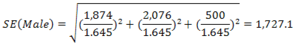
A second way is to sum the four PUMA estimates for Male to obtain:
Estimate(Male) = 5,264 + 6,508 + 4,364 + 6,865 = 23,001 as before.
The second approximation for the standard error yields:
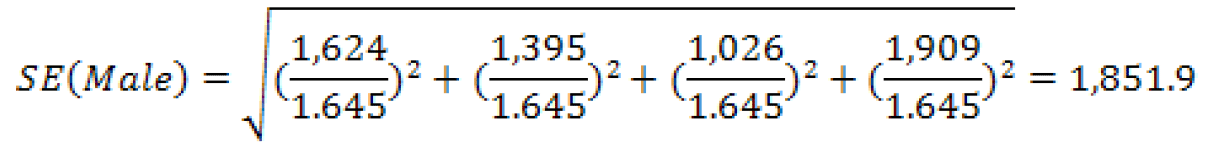
Finally, we can sum up all three age groups for all four PUMAs to obtain an estimate based on a total of twelve estimates:
Estimate(Male) = 2,041 + 2,222 + ... + 451 = 23,001
And the third approximated standard error is
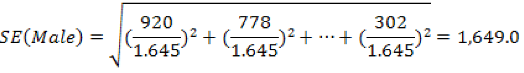
However, we do know that the standard error using the published MOE is 3,309 /1.645 = 2,011.6. In this instance, all of the approximations under-estimate the published standard error and should be used with caution.
B. Suppose we wish to estimate the total number of males at the national level using age and citizenship status. The relevant data from table B05003 is displayed in table B below.
Table B: 2009 Estimates of males from B05003: Sex by Age by Citizenship Status
The estimate and its MOE are actually published. However, if they were not available in the tables, one way of obtaining them would be to add together the number of males under 18 and over 18 to get:
Estimate (Male) = 38,146,514+ 113,223,807 = 151,375,321
And the first approximated standard error is
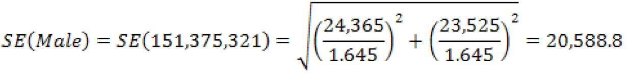
Another way would be to add up the estimates for the three subcategories (Native, and the two subcategories for Foreign Born: Naturalized U.S. Citizen, and Not a U.S. Citizen), for males under and over 18 years of age. From these six estimates we obtain:
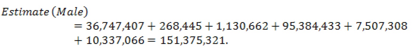
With a second approximated standard error of:
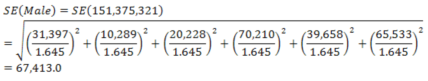
We do know that the standard error using the published margin of error is 27,279 / 1.645 = 16,583.0. With a quick glance, we can see that the ratio of the standard error of the first method to the published-based standard error yields 1.24; an over-estimate of roughly 24%, whereas the second method yields a ratio of 4.07 or an over-estimate of 307%. This is an example of what could happen to the approximate SE when the sum involves a controlled estimate. In this case, it is sex by age.
C. Suppose we are interested in the total number of people aged 65 or older and its standard error. Table C shows some of the estimates for the national level from table B01001 (the estimates in gray were derived for the purpose of this example only).
Table C: Some Estimates from AFF Table B01001: Sex by Age for 2009
To begin we find the total number of people aged 65 and over by simply adding the totals for males and females to get 16,781,175 + 22,725,542 = 39,506,717. One way we could use is summing males and female for each age category and then using their MOEs to approximate the standard error for the total number of people over 65.
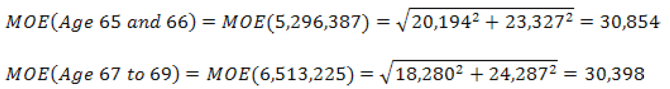
... etc. ...
Now, we calculate for the number of people aged 65 or older to be 39,506,648 using the six derived estimates and approximate the standard error:
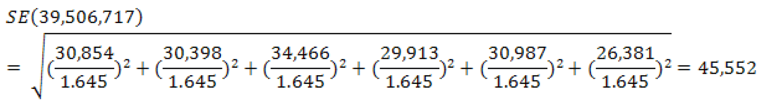
For this example the estimate and its MOE are published in table B09017. The total number of people aged 65 or older is 39,506,648 with a margin of error of 20,689. Therefore the published- based standard error is:
SE(39,506,643) = 20,689/1.645 = 12,577.
The approximated standard error, using six derived age group estimates, yields an approximated standard error roughly 3.6 times larger than the published-based standard error.
As a note, there are two additional ways to approximate the standard error of people aged 65 and over in addition to the way used above. The first is to find the published MOEs for the males age 65 and older and of females aged 65 and older separately and then combine to find the approximate standard error for the total. The second is to use all twelve of the published estimates together, that is, all estimates from the male age categories and female age categories, to create the SE for people aged 65 and older. However, in this particular example, the results from all three ways are the same. So no matter which way you use, you will obtain the same approximation for the SE. This is different from the results seen in example A.
D. For an alternative to approximating the standard error for people 65 years and older seen in part C, we could find the estimate and its SE by summing all of the estimate for the ages less than 65 years old and subtracting them from the estimate for the total population. Due to the large number of estimates, Table D does not show all of the age groups. In addition, the estimates in part of the table shaded gray were derived for the purposes of this example only and cannot be found in base table B01001.
Table D: Some Estimates from AFF Table B01001: Sex by Age for 2009:
An estimate for the number of people age 65 and older is equal to the total population minus the population between the ages of zero and 64 years old:
Number of people aged 65 and older: 307,006,556 - 267,499,908 = 39,506,648.
The way to approximate the SE is the same as in part C. First we will sum male and female estimates across each age category and then approximate the MOEs. We will use that information to approximate the standard error for our estimate of interest:
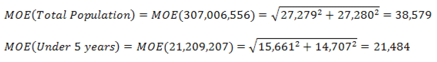
... etc. ...
And the SE for the total number of people aged 65 and older is:
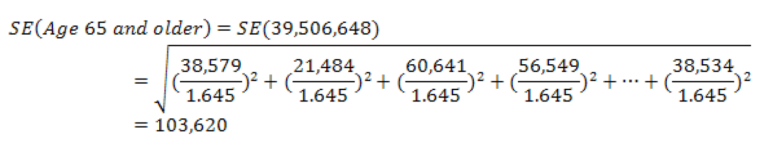
Again, as in Example C, the estimate and its MOE are we published in B09017. The total number of people aged 65 or older is 39,506,648 with a margin of error of 20,689. Therefore the standard error is:
SE(39,506,648) = 20,689 / 1.645 = 12,577.
The approximated standard error using the thirteen derived age group estimates yields a standard error roughly 8.2 times larger than the actual SE.
Data users can mitigate the problems shown in examples A through D to some extent by utilizing a collapsed version of a detailed table (if it is available) which will reduce the number of estimates used in the approximation. These issues may also be avoided by creating estimates and SEs using the Public Use Microdata Sample (PUMS) or by requesting a custom tabulation, a fee- based service offered under certain conditions by the Census Bureau. More information regarding custom tabulations may be found at http://www.census.gov/acs/www/data_documentation/custom_tabulations/.
A. Suppose we wish to estimate the total number of males with income below the poverty level in the past 12 months using both state and PUMA level estimates for the state of Wyoming. Part of the collapsed table C17001 is displayed below with estimates and their margins of error in parentheses.
Table A: 2009 Estimates of Males with Income Below Poverty from table C17001: Poverty Status in the Past 12 Months by Sex by Age
| Characteristic | Wyoming | PUMA 00100 | PUMA 00200 | PUMA 00300 | PUMA 00400 |
| Male | 23,001 (3,309) | 5,264 (1,624) | 6,508 (1,395) | 4,364 (1,026) | 6,865 (1,909) |
| Under 18 Years Old | 8,479 (1,874) | 2,041 (920) | 2,222 (778) | 1,999 (750) | 2,217 (1,192) |
| 18 to 64 Years Old | 12,976 (2,076) | 3,004 (1,049) | 3,725 (935) | 2,050 (635) | 4,197 (1,134) |
| 65 Years and Older | 1546 (500) | 219 (237) | 561 (286) | 315 (173) | 451 (302) |
| 2009 American FactFinder | |||||
The first way is to sum the three age groups for Wyoming:
Estimate(Male) = 8,479 + 12,976 + 1,546 = 23,001.
The first approximation for the standard error in this case gives us:
A second way is to sum the four PUMA estimates for Male to obtain:
Estimate(Male) = 5,264 + 6,508 + 4,364 + 6,865 = 23,001 as before.
The second approximation for the standard error yields:
Finally, we can sum up all three age groups for all four PUMAs to obtain an estimate based on a total of twelve estimates:
Estimate(Male) = 2,041 + 2,222 + ... + 451 = 23,001
And the third approximated standard error is
However, we do know that the standard error using the published MOE is 3,309 /1.645 = 2,011.6. In this instance, all of the approximations under-estimate the published standard error and should be used with caution.
B. Suppose we wish to estimate the total number of males at the national level using age and citizenship status. The relevant data from table B05003 is displayed in table B below.
Table B: 2009 Estimates of males from B05003: Sex by Age by Citizenship Status
| Characteristic | Estimate | MOE |
| Male | 151,375,321 | 27,279 |
| Under 18 Years | 38,146,514 | 24,365 |
| Native | 36,747,407 | 31,397 |
| Foreign Born | 1,399,107 | 20,177 |
| Naturalized U.S. Citizen | 268,445 | 10,289 |
| Not a U.S. Citizen | 1,130,662 | 20,228 |
| 18 Years and Older | 113,228,807 | 23,525 |
| Native | 95,384,433 | 70,210 |
| Foreign Born | 17,844,374 | 59,750 |
| Naturalized U.S. Citizen | 7,507,308 | 39,658 |
| Not a U.S. Citizen | 10,337,066 | 65,533 |
| 2009 American FactFinder | ||
The estimate and its MOE are actually published. However, if they were not available in the tables, one way of obtaining them would be to add together the number of males under 18 and over 18 to get:
Estimate (Male) = 38,146,514+ 113,223,807 = 151,375,321
And the first approximated standard error is
Another way would be to add up the estimates for the three subcategories (Native, and the two subcategories for Foreign Born: Naturalized U.S. Citizen, and Not a U.S. Citizen), for males under and over 18 years of age. From these six estimates we obtain:
With a second approximated standard error of:
We do know that the standard error using the published margin of error is 27,279 / 1.645 = 16,583.0. With a quick glance, we can see that the ratio of the standard error of the first method to the published-based standard error yields 1.24; an over-estimate of roughly 24%, whereas the second method yields a ratio of 4.07 or an over-estimate of 307%. This is an example of what could happen to the approximate SE when the sum involves a controlled estimate. In this case, it is sex by age.
C. Suppose we are interested in the total number of people aged 65 or older and its standard error. Table C shows some of the estimates for the national level from table B01001 (the estimates in gray were derived for the purpose of this example only).
Table C: Some Estimates from AFF Table B01001: Sex by Age for 2009
| Age Category | Estimate, Male | MOE, Male | Estimate, Female | MOE, Female | Total | Estimated MOE, Total |
| 65 and 66 years old | 2,492,871 | 20,194 | 2,803,516 | 23,327 | 5,296,387 | 30,854 |
| 67 to 69 years old | 3,029,709 | 18,280 | 3,483,447 | 24,287 | 6,513,225 | 30,398 |
| 70 to 74 years old | 4,088,428 | 21,588 | 4,927,666 | 26,867 | 9,016,094 | 34,466 |
| 75 to 79 years old | 3,168,175 | 19,097 | 4,204,401 | 23,024 | 7,372,576 | 29,913 |
| 80 to 84 years old | 2,258,021 | 17,716 | 3,538,869 | 25,423 | 5,796,890 | 30,987 |
| 85 years and older | 1,743,971 | 17,991 | 3,767,574 | 19,294 | 5,511,545 | 26,381 |
| Total | 16,781,175 | NA | 22,725,473 | NA | 39,506,648 | 74,932 |
| 2009 American FactFinder | ||||||
To begin we find the total number of people aged 65 and over by simply adding the totals for males and females to get 16,781,175 + 22,725,542 = 39,506,717. One way we could use is summing males and female for each age category and then using their MOEs to approximate the standard error for the total number of people over 65.
... etc. ...
Now, we calculate for the number of people aged 65 or older to be 39,506,648 using the six derived estimates and approximate the standard error:
For this example the estimate and its MOE are published in table B09017. The total number of people aged 65 or older is 39,506,648 with a margin of error of 20,689. Therefore the published- based standard error is:
SE(39,506,643) = 20,689/1.645 = 12,577.
The approximated standard error, using six derived age group estimates, yields an approximated standard error roughly 3.6 times larger than the published-based standard error.
As a note, there are two additional ways to approximate the standard error of people aged 65 and over in addition to the way used above. The first is to find the published MOEs for the males age 65 and older and of females aged 65 and older separately and then combine to find the approximate standard error for the total. The second is to use all twelve of the published estimates together, that is, all estimates from the male age categories and female age categories, to create the SE for people aged 65 and older. However, in this particular example, the results from all three ways are the same. So no matter which way you use, you will obtain the same approximation for the SE. This is different from the results seen in example A.
D. For an alternative to approximating the standard error for people 65 years and older seen in part C, we could find the estimate and its SE by summing all of the estimate for the ages less than 65 years old and subtracting them from the estimate for the total population. Due to the large number of estimates, Table D does not show all of the age groups. In addition, the estimates in part of the table shaded gray were derived for the purposes of this example only and cannot be found in base table B01001.
Table D: Some Estimates from AFF Table B01001: Sex by Age for 2009:
| Age Category | Estimate, Male | MOE, Male | Estimate, Female | MOE, Female | Total | Estimated MOE, Total |
| Total Population | 151,375,321 | 27,279 | 155,631,235 | 27,280 | 307,006,556 | 38,579 |
| Under 5 years | 10,853,263 | 15,661 | 10,355,944 | 14,707 | 21,209,207 | 21,484 |
| 5 to 9 years old | 10,273,948 | 43,555 | 9,850,065 | 42,194 | 20,124,013 | 60,641 |
| 10 to 14 years old | 10,532,166 | 40,051 | 9,985,327 | 39,921 | 20,517,493 | 56,549 |
| ... | ... | ... | ... | ... | ||
| 62 to 64 years old | 4,282,178 | 25,636 | 4,669,376 | 28,769 | 8,951,554 | 38,534 |
| Total for Age 0 to 64 years old | 134,594,146 | 117,166 | 132,905,762 | 117,637 | 267,499,908 | 166,031 |
| Total for Age 65 years and older | 16,781,175 | 120,300 | 22,725,473 | 120,758 | 39,506,648 | 170,454 |
| 2009 American FactFinder | ||||||
An estimate for the number of people age 65 and older is equal to the total population minus the population between the ages of zero and 64 years old:
Number of people aged 65 and older: 307,006,556 - 267,499,908 = 39,506,648.
The way to approximate the SE is the same as in part C. First we will sum male and female estimates across each age category and then approximate the MOEs. We will use that information to approximate the standard error for our estimate of interest:
... etc. ...
And the SE for the total number of people aged 65 and older is:
Again, as in Example C, the estimate and its MOE are we published in B09017. The total number of people aged 65 or older is 39,506,648 with a margin of error of 20,689. Therefore the standard error is:
SE(39,506,648) = 20,689 / 1.645 = 12,577.
The approximated standard error using the thirteen derived age group estimates yields a standard error roughly 8.2 times larger than the actual SE.
Data users can mitigate the problems shown in examples A through D to some extent by utilizing a collapsed version of a detailed table (if it is available) which will reduce the number of estimates used in the approximation. These issues may also be avoided by creating estimates and SEs using the Public Use Microdata Sample (PUMS) or by requesting a custom tabulation, a fee- based service offered under certain conditions by the Census Bureau. More information regarding custom tabulations may be found at http://www.census.gov/acs/www/data_documentation/custom_tabulations/.

