


| Documentation: | ACS 2009 (1-Year Estimates) |
| Document: | ACS 2009-1yr Summary File: Technical Documentation |
| citation: | Social Explorer; U.S. Census Bureau; American Community Survey 2009 Summary File: Technical Documentation. |
- Contact List: To obtain additional information on these and other American Community Survey (ACS) subjects, see the list of Census 2000/2010 Contacts on the Internet at http://www.census.gov/contacts/www/c-census2000.html.
- Scope: These definitions apply to the data collected in both the United States and Puerto Rico. The text specifically notes any differences. References about comparability to the previous ACS years refer only to the ACS in the United States. Beginning in 2006, the population in group quarters is included in the data tabulations.
- Historical Census Comparability: For additional information about the data in previous decennial censuses, see http://www.census.gov/prod/cen2000/doc/sf4.pdf.
Appendix B and subject definitions for American Community Survey years prior to 2005. - Weighting Methodology: The weighting methodology in the 2006 ACS was modified in order to ensure consistent estimates of occupied housing units, households, and householders. For more information on the 2006 weighting methodology changes, see User Notes on the ACS website (www.census.gov/acs). There were no significant changes to the 2007 or 2008 weighting methodology. Beginning in 2009, the weighting methodology has changed to include the use of controls for total population for incorporated places and minor civil divisions.
- For subject definitions from previous years, visit www.census.gov/acs.
New units not yet occupied are classified as vacant housing units if construction has reached a point where all exterior windows and doors are installed and final usable floors are in place. Vacant units are excluded from the housing inventory if they are open to the elements, that is, the roof, walls, windows, and/or doors no longer protect the interior from the elements. Also, excluded are vacant units with a sign that they are condemned or they are to be demolished.
In January 2006, the American Community Survey (ACS) was expanded to include the population living in GQ facilities. The ACS GQ sample encompasses 12 independent samples; like the housing unit (HU) sample, a new GQ sample is introduced each month. The GQ data collection lasts only 6 weeks and does not include a formal nonresponse follow-up operation. The GQ data collection operation is conducted in two phases. First, U.S. Census Bureau Field Representatives (FRs) conduct interviews with the GQ facility contact person or administrator of the selected GQ (GQ level), and second, the FR conducts interviews with a sample of individuals from the facility (person level).
The GQ-level data collection instrument is an automated Group Quarters Facility Questionnaire (GQFQ). Information collected by the FR using the GQFQ during the GQ-level interview is used to determine or verify the type of facility, population size, and the sample of individuals to be interviewed. FRs conduct GQ-level data collection at approximately 20,000 individual GQ facilities each year.
A list of the GQ facilities (and their respective type codes) that are in scope for the 2009 ACS can be found in the 2009 Code List.
In 2001, the ACS GQ operational staff and other ACS staff implemented a number of changes in the GQ operation, the greatest of which was developing an automated Group Quarters Facility Questionnaire (GQFQ). The staff developed the GQFQ based on the decennial Other Living Quarters (OLQ) questionnaire used in the 2004 Census test. However, in order to make that questionnaire script fit with the ACS operation, the developers made some modifications, such as dropping the listing component, and adding the ability to capture multiple GQ types within the special place or GQ sampled.
Along with the introduction of an automated GQFQ, the ACS made the decision to use the revised GQ definitions planned for Census 2010, even though the definitions of GQ types were still evolving. The pretest used a draft version of the GQ definitions that existed at the end of November 2004. Since these definitions will continue to evolve over the next several years, the ACS needed a GQFQ that could easily adopt future revisions to the definitions. Thus, the developers designed a flexible GQFQ. It was through this flexibility that group quarter types have been able to be added or dropped (e.g. YMCA/YWCA and hostels).
When comparing the 2009 ACS data with 2008 ACS data the data should be compared with caution at the National and State level. It should not be compared below the State level because the weighting for the group quarters (GQ) population is not controlled below the state level. Because of this users may observe greater fluctuations in year-to-year ACS estimates of the GQ population at sub-state levels than at state levels. The causes of these fluctuations typically are the result of either GQs that have closed or where the current population of the GQ is significantly different than the expected population as reflected on the sampling frame. Substantial changes in the ACS GQ estimates can impact ACS estimates of total population characteristics for areas where either the GQ population is a substantial proportion of the total population or where the GQ population may have very different characteristics than the total population as a whole. Users can assess the impact that year-to-year changes in sub-state GQ total population estimates have on the changes in total ACS population estimates by accessing Table B26001 on American Fact Finder. Users should also use their local knowledge to help determine whether the year-to-year change in the ACS estimate represents a real change in the GQ population or may be the result of the lack of adequate population controls for sub-state areas.
When comparing ACS GQ data across the years that group quarters data have been collected, it must be noted that beginning in 2008 military transient quarters, YMCA / YWCA and hostels were no longer in scope. These data were collected in 2006 and 2007.
This question determines a range of acres (cuerdas) on which the house or mobile home is located. A major purpose for this question, in conjunction with Housing Question 5 on agricultural sales, is to identify farm units. In previous American Community Surveys and in the 2000 Census, this question was used to determine single-family homes on 10 or more acres (cuerdas). The land may consist of more than one tract or plot. These tracts or plots are usually adjoining; however, they may be separated by a road, creek, another piece of land, etc. In the American Community Surveys prior to 2004 and in Census 2000, acreage was one of the variables used to determine specified owner- and renter-occupied housing units.
This question is used mainly to classify housing units as farm or nonfarm residences, not to provide detailed information on the sale of agricultural products. Detailed information on the sale of agricultural products is provided by the Census of Agriculture, which is conducted by the U.S. Department of Agriculture/National Agricultural Statistics Service (see http://www.agcensus.usda.gov/).
Bedrooms provide the basis for estimating the amount of living and sleeping spaces within a housing unit. These data allow officials to evaluate the adequacy of the housing stock to shelter the population, and to determine any housing deficiencies in neighborhoods. The data also allow officials to track the changing physical characteristics of the housing inventory over time.
In American Community Surveys prior to 2004 and in Census 2000, business on property was one of the variables used to determine specified owner- and renter-occupied housing units.
Business on property provides information on whether certain housing units should be excluded from statistics on rent, value, and shelter costs. The data provide a means to allow comparisons to be made to earlier census data by identifying information for comparable select groups of housing units without a business or medical office on the property.
Data on condominium fees may include real estate taxes and/or insurance payments for the common property, but do not include real estate taxes or fire, hazard, and flood insurance reported in Housing Questions 17 and 18 (in the 2009 American Community Survey) for the individual unit.
Amounts reported were the regular monthly payment, even if paid by someone outside the household or remain unpaid. Costs were estimated as closely as possible when exact costs were not known.
The data from this question were added to payments for mortgages (both first, second, home equity loans, and other junior mortgages); real estate taxes; fire hazard, and flood insurance payments; and utilities and fuels to derive "Selected Monthly Owner Costs" and "Selected Monthly Owner Costs as a Percentage of Household Income" for condominium owners. These data provide information on the cost of home ownership and offer an excellent measure of housing affordability and excessive shelter costs.
By listing the condominium status and fee separately on the questionnaire, the data also serve to improving the accuracy of estimating monthly housing costs for mortgaged owners.
Housing units that are renter occupied without payment of rent are shown separately as "No rent paid". The unit may be owned by friends or relatives who live elsewhere and who allow occupancy without charge. Rent-free houses or apartments may be provided to compensate caretakers, ministers, tenant farmers, sharecroppers, or others.
Contract rent is the monthly rent agreed to or contracted for, regardless of any furnishings, utilities, fees, meals, or services that may be included. For vacant units, it is the monthly rent asked for the rental unit at the time of interview.
If the contract rent includes rent for a business unit or for living quarters occupied by another household, only that part of the rent estimated to be for the respondent's unit was included. Excluded was any rent paid for additional units or for business premises.
If a renter pays rent to the owner of a condominium or cooperative, and the condominium fee or cooperative carrying charge also is paid by the renter to the owner, the condominium fee or carrying charge was included as rent.
If a renter receives payments from lodgers or roomers who are listed as members of the household, the rent without deduction for any payments received from the lodgers or roomers, was to be reported. The respondent was to report the rent agreed to or contracted for even if paid by someone else such as friends or relatives living elsewhere, a church or welfare agency, or the government through subsidies or vouchers.
Contract rent provides information on the monthly housing cost expenses for renters. When the data is used in conjunction with utility costs and income data, the information offers an excellent measure of housing affordability and excessive shelter costs. The data also serve to aid in the development of housing programs to meet the needs of people at different economic levels, and to provide assistance to agencies in determining policies on fair rent.
On October 1, 2008, the Federal Food Stamp program was renamed SNAP (Supplemental Nutrition Assistance Program). Respondents were asked if one or more of the current members received food stamps or a food stamp benefit card during the past 12 months. Respondents were also asked to include benefits from the Supplemental Nutrition Assistance Program (SNAP) in order to incorporate the program name change.
Adding the text "food stamps benefit card" to the question text and removing the dollar amount portion of the question resulted in a statistically significant increase in the recipiency rate for food stamps because of a decrease in item nonresponse rate.
Gross rent provides information on the monthly housing cost expenses for renters. When the data is used in conjunction with income data, the information offers an excellent measure of housing affordability and excessive shelter costs. The data also serve to aid in the development of housing programs to meet the needs of people at different economic levels, and to provide assistance to agencies in determining policies on fair rent.
Gross rent as a percentage of household income provides information on the monthly housing cost expenses for renters. The information offers an excellent measure of housing affordability and excessive shelter costs. The data also serve to aid in the development of housing programs to meet the needs of people at different economic levels, and to provide assistance to agencies in determining policies on fair rent.
House heating fuel is categorized on the ACS questionnaire as follows:
- Utility Gas - This category includes gas piped through underground pipes from a central system to serve the neighborhood.
- Bottled, Tank, or LP Gas - This category includes liquid propane gas stored in bottles or tanks that are refilled or exchanged when empty.
- Electricity - This category includes electricity that is generally supplied by means of above or underground electric power lines.
- Fuel Oil, Kerosene, etc. - This category includes fuel oil, kerosene, gasoline, alcohol, and other combustible liquids.
- Coal or Coke - This category includes coal or coke that is usually distributed by truck.
- Wood - This category includes purchased wood, wood cut by household members on their property or elsewhere, driftwood, sawmill or construction scraps, or the like.
- Solar Energy - This category includes heat provided by sunlight that is collected, stored, and actively distributed to most of the rooms.
- Other Fuel - This category includes all other fuels not specified elsewhere.
- No Fuel Used - This category includes units that do not use any fuel or that do not have heating equipment.
Liability policies are included only if they are paid with the fire, hazard, and flood insurance premiums and the amounts for fire, hazard, and flood cannot be separated. Premiums are reported even if they have not been paid or are paid by someone outside the household. When premiums are paid on other than a yearly basis, the premiums are converted to a yearly basis.
The payment for fire, hazard, and flood insurance is added to payments for real estate taxes, utilities, fuels, and mortgages (both first, second, home equity loans, and other junior mortgages) to derive "Selected Monthly Owner Costs" and "Selected Monthly Owner Costs as a Percentage of Household Income". These data provide information on the cost of home ownership and offer an excellent measure of housing affordability and excessive shelter costs.
A separate question (19d in the 2009 American Community Survey) determines whether insurance premiums are included in the mortgage payment to the lender(s). This makes it possible to avoid counting these premiums twice in the computations.
The meals included in rent allows for a measurement on the amount of congregate housing within the housing inventory. Congregate housing is considered to be housing units where the rent includes meals and other services.
These data include the total yearly costs for personal property taxes, land or site rent, registration fees, and license fees on all owner-occupied mobile homes. The instructions are to exclude real estate taxes already reported in Question 17 in the 2009 American Community Survey.
Costs are estimated as closely as possible when exact costs are not known. Amounts are the total for an entire 12-month billing period, even if they are paid by someone outside the household or remain unpaid.
The data from this question are added to payments for mortgages; real estate taxes; fire, hazard, and flood insurance payments; utilities; and fuels to derive "Selected Monthly Owner Costs" and "Selected Monthly Owner Costs as a Percentage of Household Income" for mobile home owners. These data provide information on the cost of home ownership and offer an excellent measure of housing affordability and excessive shelter costs.
Monthly housing costs as a percentage of household income provide information on the cost of monthly housing expenses for owners and renters. The information offers an excellent measure of housing affordability and excessive shelter costs. The data also serve to aid in the development of housing programs to meet the needs of people at different economic levels.
The amounts reported include everything paid to the lender including principal and interest payments, real estate taxes, fire, hazard, and flood insurance payments, and mortgage insurance premiums. Separate questions determine whether real estate taxes and fire, hazard, and flood insurance payments are included in the mortgage payment to the lender. This makes it possible to avoid counting these components twice in the computation of Selected Monthly Owner Costs.
Mortgage payment provides information on the monthly housing cost expenses for owners with a mortgage. When the data is used in conjunction with income data, the information offers an excellent measure of housing affordability and excessive shelter costs. The data also serve to aid in the development of housing programs aimed to meet the needs of people at different economic levels.
A mortgage is considered a first mortgage if it has prior claim over any other mortgage or if it is the only mortgage on the property. All other mortgages (second, third, etc.) are considered junior mortgages. A home equity loan is generally a junior mortgage. If no first mortgage is reported, but a junior mortgage or home equity loan is reported, then the loan is considered a first mortgage.
In most data products, the tabulations for "Selected Monthly Owner Costs" and "Selected Monthly Owner Costs as a Percentage of Household Income" usually are shown separately for units "with a mortgage" and for units "not mortgaged." The category not mortgaged is comprised of housing units owned free and clear of debt.
Mortgage status provides information on the cost of home ownership. When the data is used in conjunction with mortgage payment data, the information determines shelter costs for living quarters. These data can be use in the development of housing programs aimed to meet the needs of people at different economic levels. The data also serve to evaluate the magnitude of and to plan facilities for condominiums, which are becoming an important source of supply of new housing in many areas.
This data is the basis for estimating the amount of living and sleeping spaces within a housing unit. These data allow officials to plan and allocate funding for additional housing to relieve crowded housing conditions. The data also serve to aid in planning for future services and infrastructure, such as home energy assistance programs and the development of waste treatment facilities.
Plumbing facilities provide an indication of living standards and assess the quality of household facilities within the housing inventory. These data provide assistance in the assessment of water resources and to serve as an aid to identify possible areas of ground water contamination. The data also are used to forecast the need for additional water and sewage facilities, aid in the development of policies based on fair market rent, and to identify areas in need of rehabilitation loans or grants.
The payment for real estate taxes is added to payments for fire, hazard, and flood insurance; utilities and fuels; and mortgages (both first and second mortgages, home equity loans, and other junior mortgages) to derive "Selected Monthly Owner Costs" and "Selected Monthly Owner Costs as a Percentage of Household Income". These data provide information on the cost of home ownership and offer an excellent measure of housing affordability and excessive shelter costs. A separate question (Question 19c in the 2008 American Community Survey) determines whether real estate taxes are included in the mortgage payment to the lender(s). This makes it possible to avoid counting taxes twice in the computations.
For each unit, rooms include living rooms, dining rooms, kitchens, bedrooms, finished recreation rooms, enclosed porches suitable for year-round use, and lodger's rooms. Excluded are strip or pullman kitchens, bathrooms, open porches, balconies, halls or foyers, half-rooms, utility rooms, unfinished attics or basements, or other unfinished space used for storage. A partially divided room is a separate room only if there is a partition from floor to ceiling, but not if the partition consists solely of shelves or cabinets.
Rooms provide the basis for estimating the amount of living and sleeping spaces within a housing unit. These data allow officials to plan and allocate funding for additional housing to relieve crowded housing conditions. The data also serve to aid in planning for future services and infrastructure, such as home energy assistance programs and the development of waste treatment facilities.
All mortgages other than first mortgages (for example, second, third, etc.) are classified as "junior" mortgages. A second mortgage is a junior mortgage that gives the lender a claim against the property that is second to the claim of the holder of the first mortgage. Any other junior mortgage(s) would be subordinate to the second mortgage. A home equity loan is a line of credit available to the borrower that is secured by real estate. It may be placed on a property that already has a first or second mortgage, or it may be placed on a property that is owned free and clear.
If the respondents answered that no first mortgage existed, but a second mortgage or a home equity loan did, a computer edit assigned the unit a first mortgage and made the first mortgage monthly payment the amount reported in the second mortgage. The second mortgage/home equity loan data were then made "No" in Question 20a and blank in Question 20b.
Second mortgage or home equity loan data provide information on the monthly housing cost expenses for owners. When the data is used in conjunction with income data, the information offers an excellent measure of housing affordability and excessive shelter costs. The data also serve to aid in the development of housing programs aimed to meet the needs of people at different economic levels.
By listing the second mortgage or home equity loan question separately on the questionnaire from other housing cost questions, the data also serve to improving the accuracy of estimating monthly housing costs for mortgaged owners.
1) lacking complete plumbing facilities,
2) lacking complete kitchen facilities,
3) with 1.01 or more occupants per room,
4) selected monthly owner costs as a percentage of household income greater than 30 percent, and
5) gross rent as a percentage of household income greater than 30 percent. Selected conditions provide information in assessing the quality of the housing inventory and its occupants. The data is used to easily identify those homes in which the quality of living and housing can be considered substandard.
Selected monthly owner costs provide information on the monthly housing cost expenses for owners. When the data is used in conjunction with income data, the information offers an excellent measure of housing affordability and excessive shelter costs. The data also serve to aid in the development of housing programs to meet the needs of people at different economic levels.
Separate distributions are often shown for units "with a mortgage" and for units "not mortgaged." Units occupied by households reporting no income or a net loss are included in the ''not computed" category. (For more information, see the discussion under "Selected Monthly Owner Costs.")
Selected monthly owner costs as a percentage of household income provide information on the monthly housing cost expenses for owners. The information offers an excellent measure of housing affordability and excessive shelter costs. The data also serve to aid in the development of housing programs to meet the needs of people at different economic levels.
Specified owner-occupied unit information is used to maintain a comparable universe between the American Community Survey and earlier census data. Financial housing characteristics in earlier census data were based on a specified owner-occupied unit, however the ACS does not provide information solely for this universe. Therefore, the characteristics for a specified owner-occupied unit are maintained within the PUMS file to ensure comparisons can be made between the two data sets.
The question asked whether telephone service was available in the house, apartment, or mobile home. A telephone must be in working order and service available in the house, apartment, or mobile home that allows the respondent to both make and receive calls. Households whose service has been discontinued for nonpayment or other reasons are not counted as having telephone service available.
The availability of telephone service provides information on the isolation of households. These data help assess the level of communication access amongst elderly and low-income households. The data also serve to aid in the development of emergency telephone, medical, or crime prevention services.
Tenure provides a measurement of home ownership, which has served as an indicator of the nations economy for decades. These data are used to aid in the distribution of funds for programs such as those involving mortgage insurance, rental housing, and national defense housing. Data on tenure allows planners to evaluate the overall viability of housing markets and to assess the stability of neighborhoods. The data also serve in understanding the characteristics of owner occupied and renter occupied units to aid builders, mortgage lenders, planning officials, government agencies, etc., in the planning of housing programs and services.
A housing unit is "Owned by you or someone in this household free and clear (without a mortgage or loan)" if there is no mortgage or other similar debt on the house, apartment, or mobile home including units built on leased land if the unit is owned outright without a mortgage.
The units in structure provides information on the housing inventory by subdividing the inventory into one-family homes, apartments, and mobile homes. When the data is used in conjunction with tenure, year structure built, and income, units in structure serves as the basic identifier of housing used in many federal programs. The data also serve to aid in the planning of roads, hospitals, utility lines, schools, playgrounds, shopping centers, emergency preparedness plans, and energy consumption and supplies.
Costs are recorded if paid by or billed to occupants, a welfare agency, relatives, or friends. Costs that are paid by landlords, included in the rent payment, or included in condominium or cooperative fees are excluded.
The cost of utilities provides information on the cost of either home ownership or renting. When the data is used as part of monthly housing costs and in conjunction with income data, the information offers an excellent measure of housing affordability and excessive shelter costs. The data also serve to aid in the development of housing programs to meet the needs of people at different economic levels, and to provide assistance in forecasting future utility services and energy supplies.
Vacant units are subdivided according to their housing market classification as follows:
The year the structure was built provides information on the age of housing units. These data help identify new housing construction and measures the disappearance of old housing from the inventory, when used in combination with data from previous years. The data also serve to aid in the development of formulas to determine substandard housing and provide assistance in forecasting future services, such as energy consumption and fire protection.
Government agencies use information on language spoken at home for their programs that serve the needs of the foreign-born and specifically those who have difficulty with English. Under the Voting Rights Act, language is needed to meet statutory requirements for making voting materials available in minority languages. The Census Bureau is directed, using data about language spoken at home and the ability to speak English, to identify minority groups that speak a language other than English and to assess their English-speaking ability. The U.S. Department of Education uses these data to prepare a report to Congress on the social and economic status of children served by different local school districts.
Government agencies use information on language spoken at home for their programs that serve the needs of the foreign-born and specifically those who have difficulty with English. Under the Voting Rights Act, language is needed to meet statutory requirements for making voting materials available in minority languages. The Census Bureau is directed, using data about language spoken at home and the ability to speak English, to identify minority groups that speak a language other than English and to assess their English-speaking ability. The U.S. Department of Education uses these data to prepare a report to Congress on the social and economic status of children served by different local school districts. State and local agencies concerned with aging develop health care and other services tailored to the language and cultural diversity of the elderly under the Older Americans Act.
Age is asked for all person's in a household or group quarters. On the mailout/mailback paper questionnaire for households, both age and date of birth are asked for person's listed as person numbers 1-5 on the form. Only age (in years) is initially asked for person's listed as 6-12 on the mailout/mailback paper questionnaire. If a respondent indicates that there are more than 5 people living in the household, then the household is eligible for Failed Edit Follow-up (FEFU). During FEFU operations, telephone center staffers call respondents to obtain missing data. This includes asking date of birth for any person in the household missing date of birth information. In Computer Assisted Telephone Interviews (CATI) and Computer Assisted Personal Interview (CAPI) instruments both age and date of birth is asked for all person's. In 2006, the ACS began collecting data in group quarters (GQs). This included asking both age and date of birth for person's living in a group quarters. For additional data collection methodology, please see www.census.gov/acs.
Data on age are used to determine the applicability of other questions for a particular individual and to classify other characteristics in tabulations. Age data are needed to interpret most social and economic characteristics used to plan and analyze programs and policies. Age is central for any number of federal programs that target funds or services to children, working-age adults, women of childbearing age, or the older population. The U.S. Department of Education uses census age data in its formula for allotment to states. The U.S. Department of Veterans Affairs uses age to develop its mandated state projections on the need for hospitals, nursing homes, cemeteries, domiciliary services, and other benefits for veterans. For more information on the use of age data in Federal programs, please see www.census.gov/acs.
Data users should also be aware of methodology differences that may exist between different data sources if they are comparing American Community Survey age data to data sources, such as Population Estimates or Decennial Census data. For example, the American Community Survey data are that of a respondent-based survey and subject to various quality measures, such as sampling and nonsampling error, response rates and item allocation error. This differs in design and methodology from other data sources, such as Population Estimates, which is not a survey and involves computational methodology to derive intercensal estimates of the population. While ACS estimates are controlled to Population Estimates for age at the nation, state and county levels of geography as part of the ACS weighting procedure, variation may exist in the age structure of a population at lower levels of geography when comparing different time periods or comparing across time due to the absence of controls below the county geography level. For more information on American Community Survey data accuracy and weighting procedures, please see www.census.gov/acs.
It should also be noted that although the American Community Survey (ACS) produces population, demographic and housing unit estimates, it is the Census Bureau's Population Estimates Program that produces and disseminates theofficial estimates of the population for the nation, states, counties, cities and towns and estimates of housing units for states and counties. (Please refer to: factfinder.census.gov/home/en/official_estimates_2008.html)
The intent of the ancestry question was not to measure the degree of attachment the respondent had to a particular ethnicity, but simply to establish that the respondent had a connection to and self-identified with a particular ethnic group. For example, a response of "Irish" might reflect total involvement in an Irish community or only a memory of ancestors several generations removed from the individual.
The data on ancestry were derived from answers to Question 13. The question was based on self-identification; the data on ancestry represent self-classification by people according to the ancestry group(s) with which they most closely identify.
The Census Bureau coded the responses into a numeric representation of over 1,000 categories. To do so, responses initially were processed through an automated coding system; then, those that were not automatically assigned a code were coded by individuals trained in coding ancestry responses. The code list reflects the results of the Census Bureau's own research and consultations with many ethnic experts. Many decisions were made to determine the classification of responses. These decisions affected the grouping of the tabulated data. For example, the Indonesian category includes the responses of "Indonesian," "Celebesian," "Moluccan," and a number of other responses.
The ancestry question allowed respondents to report one or more ancestry groups. Generally, only the first two responses reported were coded. If a response was in terms of a dual ancestry, for example, "Irish English," the person was assigned two codes, in this case one for Irish and another for English. However, in certain cases, multiple responses such as "French Canadian," "Scotch-Irish," "Greek Cypriot," and "Black Dutch" were assigned a single code reflecting their status as unique groups. If a person reported one of these unique groups in addition to another group, for example, "Scotch-Irish English," resulting in three terms, that person received one code for the unique group (Scotch-Irish) and another one for the remaining group (English). If a person reported "English Irish French," only English and Irish were coded. For certain combinations of ancestries where the ancestry group is a part of another, such as "German Bavarian," the responses were coded as a single ancestry using the more detailed group (Bavarian). Also, responses such as "Polish-American" or "Italian-American" were coded and tabulated as a single entry (Polish or Italian).
The Census Bureau accepted "American" as a unique ethnicity if it was given alone, with an ambiguous response, or with state names. If the respondent listed any other ethnic identity such as "Italian American," generally the "American" portion of the response was not coded. However, distinct groups such as "American Indian," "Mexican American," and "African American" were coded and identified separately because they represented groups who may consider themselves different from those who reported as "Indian," "Mexican," or "African," respectively.
The ancestry question is asked for every person in the American Community Survey, regardless of age, place of birth, "Hispanic" origin, or race.
Ancestry identifies the ethnic origins of the population, and Federal agencies regard this information as essential for fulfilling many important needs. Ancestry is required to enforce provisions under the Civil Rights Act, which prohibits discrimination based upon race, sex, religion, and national origin. More generally, these data are needed to measure the social and economic characteristics of ethnic groups and to tailor services to accommodate cultural differences. The Department of Labor draws samples for surveys that provide employment statistics and other related information for ethnic groups using ancestry.
The ACS data on ancestry are released annually on the Census Bureau's internet site. The Detailed Tables (B04001-B04007) contain estimates of over 100 different ancestry groups for the nation, states, and many other geographic areas, while the Special Population Profiles contain characteristics of different ancestry groups.
In all tabulations, when respondents provided an unclassifiable ethnic identity (for example, "multi-national," "adopted," or "I have no idea"), the answer was included in "Unclassified or not reported."
The tabulations on ancestry show two types of data- one where estimates represent the number of people, and the other where estimates represent the number of responses. If you want to know how many people reported an ancestry, use the estimates based on people. If you want to know how many reports there were of a certain ancestry, use the estimates based on reports. The difference between the two types of data presentations represents the fact that people can provide more than one ancestry, therefore can be counted twice in the same ancestry category. Examples are provided below.
The following are the types of estimates shown:
The question on ancestry was first asked in the 1980 Census. It replaced the question on parental place of birth, in order to include ancestral heritage for people whose families have been in the U.S. for more than two generations. The question was also asked in the 1990 and 2000 censuses.
From 1996 to 1999, the ACS editing system used answers to the race and place of birth questions to clarify ancestry responses of "Indian," where possible. In 2000 and subsequent years, the editing was expanded to aid interpretation of two-word ancestries, such as "Black Irish."
Beginning in 2006, the population in group quarters (GQ) was included in the ACS. Some types of GQ populations may have ancestry distributions that are different from the household population. The inclusion of the GQ population could therefore have a noticeable impact on the ancestry distribution. This is particularly true for areas with a substantial GQ population.
Data were most frequently presented in terms of the aggregate number of children ever born to women in the specified category and in terms of the rate per 1,000 women.
Beginning in 1999, American Community Survey data on fertility were derived from questions that asked if the person had given birth in the past 12 months. See the section on Fertility for more information.
Respondents were asked to select one of five categories: (1) born in the United States, (2) born in Puerto Rico, Guam, the U.S. Virgin Islands, or Northern Marianas, (3) born abroad of U.S. citizen parent or parents, (4) U.S. citizen by naturalization, or (5) not a U.S citizen. Respondents indicating they are a U.S. citizen by naturalization are also asked to print their year of naturalization. People born in American Samoa, although not explicitly listed, are included in the second response category.
For the Puerto Rico Community Survey, respondents were asked to select one of five categories: (1) born in Puerto Rico, (2) born in a U.S. state, District of Columbia, Guam, the U.S. Virgin Islands, or Northern Marianas, (3) born abroad of U.S. citizen parent or parents, (4) U.S. citizen by naturalization, or (5) not a U.S. citizen. Respondents indicating they are a U.S. citizen by naturalization are also asked to print their year of naturalization. People born in American Samoa, although not explicitly listed, are included in the second response category.
When no information on citizenship status was reported for a person, information for other household members, if available, was used to assign a citizenship status to the respondent. All cases of nonresponse that were not assigned a citizenship status based on information from other household members were allocated the citizenship status of another person with similar characteristics who provided complete information. In cases of conflicting responses, place of birth information is used to edit citizenship status. For example, if a respondent states he or she was born in Puerto Rico but was not a U.S. citizen, the edits use the response to the place of birth question to change the respondents status to "U.S. citizen at birth."
- An employee of a private, for-profit company or business, or of an individual, for wages, salary, or commissions.
- An employee of a private, not-for-profit, tax-exempt, or charitable organization.
- A local government employee (city, county, etc.).
- A state government employee.
- A Federal government employee.
- Self-employed in own not incorporated business, professional practice, or farm.
- Self-employed in own incorporated business, professional practice, or farm.
- Working without pay in a family business or farm.
These questions were asked of all people 15 years old and over who had worked in the past 5 years. For employed people, the data refer to the person's job during the previous week. For those who worked two or more jobs, the data refer to the job where the person worked the greatest number of hours. For unemployed people and people who are not currently employed but report having a job within the last five years, the data refer to their last job. The class of worker categories are defined as follows:
ACS tabulations present data separately for these subcategories: "Employee of private company workers," "Private not-for-profit wage and salary workers," and "Self-employed in own incorporated business workers."
The government categories include all government workers, though government workers may work in different industries. For example, people who work in a public elementary school or city owned bus line are coded as local government class of workers.
Self-employed in own not incorporated business workers - Includes people who worked for profit or fees in their own unincorporated business, profession, or trade, or who operated a farm.
These data are used to formulate policy and programs for employment and career development and training. Companies use these data to decide where to locate new plants, stores, or offices.
Data on occupation, industry, and class of worker are collected for the respondents current primary job or the most recent job for those who are not employed but have worked in the last 5 years. Other labor force questions, such as questions on earnings or work hours, may have different reference periods and may not limit the response to the primary job. Although the prevalence of multiple jobs is low, data on some labor force items may not exactly correspond to the reported occupation, industry, or class of worker of a respondent.
Furthermore, disability is a dynamic concept that changes over time as ones health improves or declines, as technology advances, and as social structures adapt. As such, disability is a continuum in which the degree of difficulty may also increase or decrease. Because disability exists along a continuum, various cut-offs are used to allow for a simpler understanding of the concept, the most common of which is the dichotomous "With a disability"/"no disability" differential.
Measuring this complex concept of disability with a short set of six questions is difficult. Because of the multitude of possible functional limitations that may present as disabilities, and in the absence of information on external factors that influence disability, surveys like the ACS are limited to capturing difficulty with only selected activities. As such, people identified by the ACS as having a disability are, in fact, those who exhibit difficulty with specific functions and may, in the absence of accommodation, have a disability. While this definition is different from the one described by the IOM and ICF conceptual frameworks, it relates to the programmatic definitions used in most Federal and state legislation.
In an attempt to capture a variety of characteristics that encompass the definition of disability, the ACS identifies serious difficulty with four basic areas of functioning - hearing, vision, cognition, and ambulation. These functional limitations are supplemented by questions about difficulties with selected activities from the Katz Activities of Daily Living (ADL) and Lawton Instrumental Activities of Daily Living (IADL) scales, namely difficulty bathing and dressing, and difficulty performing errands such as shopping. Overall, the ACS attempts to capture six aspects of disability, which can be used together to create an overall disability measure, or independently to identify populations with specific disability types.
Information on disability is used by a number of federal agencies to distribute funds and develop programs for people with disabilities. For example, data about the size, distribution, and needs of the disabled population are essential for developing disability employment policy. For the Americans with Disabilities Act, data about functional limitations are important to ensure that comparable public transportation services are available for all segments of the population. Federal grants are awarded, under the Older Americans Act, based on the number of elderly people with physical and mental disabilities.
Disability status is determined from the answers from these six types of difficulty. For children under 5 years old, hearing and vision difficulty are used to determine disability status. For children between the ages of 5 and 14, disability status is determined from hearing, vision, cognitive, ambulatory, and self-care difficulties. For people aged 15 years and older, they are considered to have a disability if they have difficulty with any one of the six difficulty types.
The 2009 disability estimates should also not be compared with disability estimates from Census 2000 for reasons similar to the ones made above. ACS disability estimates should also not be compared with more detailed measures of disability from sources such as the National Health Interview Survey and the Survey of Income and Program Participation.
The 2009 ACS disability estimates are comparable with the ACS disability estimates from 2008.
Data on educational attainment were derived from answers to Question 11, which was asked of all respondents. Educational attainment data are tabulated for people 18 years old and over. Respondents are classified according to the highest degree or the highest level of school completed. The question included instructions for persons currently enrolled in school to report the level of the previous grade attended or the highest degree received.
The educational attainment question included a response category that allowed people to report completing the 12th grade without receiving a high school diploma. Respondents who received a regular high school diploma and did not attend college were instructed to report "Regular high school diploma". Respondents who received the equivalent of a high school diploma (for example, passed the test of General Educational Development (G.E.D.)), and did not attend college, were instructed to report "GED or alternative credential."
"Some college" is in two categories: "Some college credit, but less than 1 year of college credit" and "1 or more years of college credit, no degree." The category "Associate's degree" included people whose highest degree is an associates degree, which generally requires 2 years of college level work and is either in an occupational program that prepares them for a specific occupation, or an academic program primarily in the arts and sciences. The course work may or may not be transferable to a bachelor's degree. Master's degrees include the traditional MA and MS degrees and field-specific degrees, such as MSW, MEd, MBA, MLS, and MEng. Instructions included in the respondent instruction guide for mailout/mailback respondents only provided the following examples of professional school degrees: Medicine, dentistry, chiropractic, optometry, osteopathic medicine, pharmacy, podiatry, veterinary medicine, law, and theology. The order in which degrees were listed suggested that doctorate degrees were "higher" than professional school degrees, which were "higher" than master's degrees. If more than one box was filled, the response was edited to the highest level or degree reported.
The instructions further specified that schooling completed in foreign or ungraded school systems should be reported as the equivalent level of schooling in the regular American system. The instructions specified that certificates or diplomas for training in specific trades or from vocational, technical or business schools were not to be reported. Honorary degrees awarded for a respondent's accomplishments were not to be reported.
In the 1996-1998 American Community Survey, the educational attainment question was used to estimate level of enrollment. Since 1999, a question regarding grade of enrollment was included.
The 1999-2007 American Community Survey attainment question grouped grade categories below high school into the following three categories: "Nursery school to 4th grade," "5th grade or 6th grade," and "7th grade or 8th grade." The 1996-1998 American Community Survey question allowed a write-in for highest grade completed for grades 1-11 in addition to "Nursery or preschool" and "Kindergarten."
Beginning in 2008, the American Community Survey attainment question was changed to the following categories for levels up to ""Grade 12, no diploma:" "Nursery school," "Kindergarten," "Grade 1 through grade 11," and "12th grade, no diploma." The survey question allowed a write-in for the highest grade completed for grades 1-11. In addition, the category that was previously "High school graduate (including GED)" was broken into two categories: "Regular high school diploma" and "GED or alternative credential." The term credit for the two some college categories was emphasized. The phrase beyond a bachelor's degree was added to the professional degree category.
Data about educational attainment are also collected from the decennial Census and from the Current Population Survey (CPS). ACS data is generally comparable to data from the Census. For more information about the comparability of ACS and CPS data, please see the link for the Fact Sheet and the Comparison Report from the CPS Educational Attainment page.
The employment status data shown in American Community Survey tabulations relate to people 16 years old and over.
Employment status is key to understanding work and unemployment patterns and the availability of workers. Based on labor market areas and unemployment levels, the U.S. Department of Labor identifies service delivery areas and determines amounts to be allocated to each for job training. The impact of immigration on the economy and job markets is determined partially by labor force data, and this information is included in required reports to Congress. The Office of Management and Budget, under the Paperwork Reduction Act, uses data about employed workers as part of the criteria for defining metropolitan areas. The Bureau of Economic Analysis uses this information, in conjunction with other data, to develop its state per capita income estimates used in the allocation formulas and eligibility criteria for many federal programs such as Medicaid.
- Registering at a public or private employment office
- Meeting with prospective employers
- Investigating possibilities for starting a professional practice or opening a business
- Placing or answering advertisements
- Writing letters of application
- Being on a union or professional register
On Layoff (Question 35a): Starting in 1999, the "Yes, on temporary layoff from most recent job" and "Yes, permanently laid off from most recent job" response categories were condensed into a single "Yes" category. An additional question (Q35b) was added to determine the temporary/permanent layoff distinction. Temporarily Absent (Question 35b): Starting in 2008, the temporarily absent question included a revised list of examples of work absences.
Recalled to Work (Question 35c): This question was added in the 1999 American Community Survey to determine if a respondent who reported being on layoff from a job had been informed that he or she would be recalled to work within 6 months or been given a date to return to work.
Looking for Work (Question 36): Starting in 2008, the actively looking for work question was modified to emphasize 'active' job-searching activities.
Available to Work (Question 37): Starting in 1999, the "Yes, if a job had been offered" and "Yes, if recalled from layoff" response categories were condensed into one category, "Yes, could have gone to work." Starting in 2008, the actively looking for work question was modified to emphasize 'active' job-searching activities.
Beginning in 2006, the population in group quarters (GQ) is included in the ACS. Some types of GQ populations have employment status distributions that are different from the household population. All institutionalized people are placed in the not in labor force category. The inclusion of the GQ population could therefore have a noticeable impact on the employment status distribution. This is particularly true for areas with a substantial GQ population. For example, in areas having a large state prison population, the employment rate would be expected to decrease because the base of the percentage, which now includes the population in correctional institutions, is larger. The Census Bureau tested the changes introduced to the 2008 version of the employment status questions in the 2006 ACS Content Test. The results of this testing show that the changes may introduce an inconsistency in the data produced for these questions as observed from the years 2007 to 2008, see "2006 ACS Content Test Evaluation Report Covering Employment Status" on the ACS website (www.census.gov/acs).
Along with the 2008 ACS release, the Census Bureau produced a research note comparing 2007 and 2008 ACS employment estimates to 2007 and 2008 Current Population Survey (CPS)/Local Area Unemployment Statistics (LAUS) estimates. The research note shows that the changes to the employment status series of questions in the 2008 ACS will make ACS labor force data more consistent with benchmark data from the CPS and LAUS program. For more information, see "Changes to the American Community Survey between 2007 and 2008 and the Effects on the Estimates of Employment and Unemployment" (http://www.census.gov/hhes/www/laborfor/researchnote092209.html).
An additional difference in the data arises from the fact that people who had a job but were not at work are included with the employed in the American Community Survey statistics, whereas many of these people are likely to be excluded from employment figures based on establishment payroll reports. Furthermore, the employment status data in tabulations include people on the basis of place of residence regardless of where they work, whereas establishment data report people at their place of work regardless of where they live. This latter consideration is particularly significant when comparing data for workers who commute between areas.
For several reasons, the unemployment figures of the Census Bureau are not comparable with published figures on unemployment compensation claims. For example, figures on unemployment compensation claims exclude people who have exhausted their benefit rights, new workers who have not earned rights to unemployment insurance, and people losing jobs not covered by unemployment insurance systems (including some workers in agriculture, domestic services, and religious organizations, and self-employed and unpaid family workers). In addition, the qualifications for drawing unemployment compensation differ from the definition of unemployment used by the Census Bureau. People working only a few hours during the week and people "with a job but not at work" are sometimes eligible for unemployment compensation but are classified as "Employed" in the American Community Survey. Differences in the geographical distribution of unemployment data arise because the place where claims are filed may not necessarily be the same as the place of residence of the unemployed worker.
For guidance on differences in employment and unemployment estimates from different sources, go to http://www.census.gov/hhes/www/laborfor/laborguidance082504.html.
An automated computer system coded write-in responses to Question 12 into 192 areas. Clerical coding categorized any write-in responses that could not be autocoded by the computer. Respondents listing multiple fields were assigned a code for each field, with a maximum of 10 fields per respondent. The majors were further classified into a category scheme detailed in Appendix A.
- Insurance through a current or former employer or union (of this person or another family member)
- Insurance purchased directly from an insurance company (by this person or another family member)
- Medicare, for people 65 and older, or people with certain disabilities
- Medicaid, Medical Assistance, or any kind of government-assistance plan for those with low incomes or a disability
- TRICARE or other military health care
- VA (including those who have ever used or enrolled for VA health care)
- Indian Health Service
- Any other type of health insurance or health coverage plan
Respondents who answered "yes" to question 16h were asked to provide their other type of coverage type in a write-in field.
Health insurance coverage in the ACS and other Census Bureau surveys define coverage to include plans and programs that provide comprehensive health coverage. Plans that provide insurance for specific conditions or situations such as cancer and long-term care policies are not considered coverage. Likewise, other types of insurance like dental, vision, life, and disability insurance are not considered health insurance coverage.
In defining types of coverage, write-in responses were reclassified into one of the first seven types of coverage or determined not to be a coverage type. Write-in responses that referenced the coverage of a family member were edited to assign coverage based on responses from other family members. As a result, only the first seven types of health coverage are included in the microdata file.
An eligibility edit was applied to give Medicaid, Medicare, and TRICARE coverage to individuals based on program eligibility rules. TRICARE or other military health care was given to active-duty military personnel and their spouses and children. Medicaid or other means-tested public coverage was given to foster children, certain individuals receiving Supplementary Security Income or Public Assistance, and the spouses and children of certain Medicaid beneficiaries. Medicare coverage was given to people 65 and older who received Social Security or Medicaid benefits.
People were considered insured if they reported at least one "yes" to Questions 16a to 16f. People who had no reported health coverage, or those whose only health coverage was Indian Health Service, were considered uninsured. For reporting purposes, the Census Bureau broadly classifies health insurance coverage as private health insurance or public coverage. Private health insurance is a plan provided through an employer or union, a plan purchased by an individual from a private company, or TRICARE or other military health care. Respondents reporting a "yes" to the types listed in parts a, b, or e were considered to have private health insurance. Public health coverage includes the federal programs Medicare, Medicaid, and VA Health Care (provided through the Department of Veterans Affairs); the Childrens Health Insurance Program (CHIP); and individual state health plans. Respondents reporting a "yes" to the types listed in c, d, or f were considered to have public coverage. The types of health insurance are not mutually exclusive; people may be covered by more than one at the same time.
The U.S. Department of Health and Human Services, as well as other federal agencies, use data on health insurance coverage to more accurately distribute resources and better understand state and local health insurance needs.
For the 2008 data released September 2009, there was no eligibility edit applied. The eligibility edit that was developed for the 2009 was applied to the 2008 data during spring 2010. New estimates of health insurance coverage with this data are available at http://www.census.gov/hhes/www/hlthins/hlthins.html.
Because coverage in the ACS references an individual's current status, caution should be taken when making comparisons to other surveys which may define coverage as "at any time in the last year" or "throughout the past year." A discussion of how the ACS health insurance estimates relate to other survey health insurance estimates can be found in "A Preliminary Evaluation of Health Insurance Coverage" in the 2008 American Community Survey (http://www.census.gov/hhes/www/hlthins/acs08paper/2008ACS_healthins.pdf).
Origin can be viewed as the heritage, nationality group, lineage, or country of birth of the person or the person's parents or ancestors before their arrival in the United States. People who identify their origin as "Hispanic", "Latino," or "Spanish" may be of any race.
Hispanic origin is used in numerous programs and is vital in making policy decisions. These data are needed to determine compliance with provisions of antidiscrimination in employment and minority recruitment legislation. Under the Voting Rights Act, data about Hispanic origin are essential to ensure enforcement of bilingual election rules. Hispanic origin classifications used by the Census Bureau and other federal agencies meet the requirements of standards issued by the Office of Management and Budget in 1997 (Revisions to the Standards for the Classification of Federal Data on Race and Ethnicity). These standards set forth guidance for statistical collection and reporting on race and ethnicity used by all federal agencies.
Some tabulations are shown by the origin of the householder. In all cases where the origin of households, families, or occupied housing units is classified as Hispanic, Latino, or Spanish, the origin of the householder is used. (For more information, see the discussion of householder under "Household Type and Relationship.")
The responses to this question were used to determine the relationships of all persons to the householder, as well as household type (married couple family, nonfamily, etc.). From responses to this question, we were able to determine numbers of related children, own children, unmarried partner households, and multigenerational households. We calculated average household and family size. When relationship was not reported, it was imputed using the age difference between the householder and the person, sex, and marital status.
- Biological son or daughter - The son or daughter of the householder by birth.
- Adopted son or daughter - The son or daughter of the householder by legal adoption. If a stepson or stepdaughter has been legally adopted by the householder, the child is then classified as an adopted child.
- Stepson or stepdaughter - The son or daughter of the householder through marriage but not by birth, excluding sons-in-law and daughters-in-law. If a stepson or stepdaughter of the householder has been legally adopted by the householder, the child is then classified as an adopted child.
- Grandchild - The grandson or granddaughter of the householder.
- Brother/Sister - The brother or sister of the householder, including stepbrothers, stepsisters, and brothers and sisters by adoption. Brothers-in-law and sisters-in-law are included in the "Other Relative" category on the questionnaire.
- Parent - The father or mother of the householder, including a stepparent or adoptive parent. Fathers-in-law and mothers-in-law are included in the "Parent-in-law" category on the questionnaire.
- Parent-in-law - The mother-in-law or father-in-law of the householder.
- Son-in-law or daughter-in-law - The spouse of the child of the householder.
- Other Relatives - Anyone not listed in a reported category above who is related to the householder by birth, marriage, or adoption (brother-in-law, grandparent, nephew, aunt, cousin, and so forth).
- Roomer or Boarder - A roomer or boarder is a person who lives in a room in the household of the householder. Some sort of cash or noncash payment (e.g., chores) is usually made for their living accommodations.
- Housemate or Roommate - A housemate or roommate is a person age 15 years and over, who is not related to the householder, and who shares living quarters primarily in order to share expenses.
- Unmarried Partner - An unmarried partner is a person age 15 years and over, who is not related to the householder, who shares living quarters, and who has a close personal relationship with the householder. Same-sex spouses are included in this category for tabulation purposes and for public use data files.
- Foster Child - A foster child is a person who is under 21 years old placed by the local government in a household to receive parental care. Foster children may be living in the household for just a brief period or for several years. Foster children are nonrelatives of the householder. If the foster child is also related to the householder, the child is classified as that specific relative.
- Other Nonrelatives - Anyone who is not related by birth, marriage, or adoption to the householder and who is not described by the categories given above.
When relationship is not reported for an individual, it is imputed according to the responses for age, sex, and marital status for that person while maintaining consistency with responses for other individuals in the household.
- Married-Couple Family - A family in which the householder and his or her spouse are listed as members of the same household.
- Other Family: Male Householder, No Wife Present - A family with a male householder and no spouse of householder present.
- Female Householder, No Husband Present - A family with a female householder and no spouse of householder present.
Family households and married-couple families do not include same-sex married couples even if the marriage was performed in a state issuing marriage certificates for same-sex couples. Same sex couple households are included in the family households category if there is at least one additional person related to the householder by birth or adoption.
In some labor force tabulations, children in both one-parent families and one-parent subfamilies are included in the total number of children living with one parent, while children in both married-couple families and married-couple subfamilies are included in the total number of children living with two parents.
Receipts from the following sources are not included as income: capital gains, money received from the sale of property (unless the recipient was engaged in the business of selling such property); the value of income "in kind" from food stamps, public housing subsidies, medical care, employer contributions for individuals, etc.; withdrawal of bank deposits; money borrowed; tax refunds; exchange of money between relatives living in the same household; gifts and lump-sum inheritances, insurance payments, and other types of lump-sum receipts.
Income is a vital measure of general economic circumstances. Income data are used to determine poverty status, to measure economic well-being, and to assess the need for assistance. These data are included in federal allocation formulas for many government programs. For instance:
Social Services: Under the Older Americans Act, funds for food, health care, and legal services are distributed to local agencies based on data about elderly people with low incomes. Data about income at the state and county levels are used to allocate funds for food, health care, and classes in meal planning to low-income women with children.
Employment: Income data are used to identify local areas eligible for grants to stimulate economic recovery, run job-training programs, and define areas such as empowerment or enterprise zones.
Housing: Under the Low-Income Home Energy Assistance Program, income data are used to allocate funds to areas for home energy aid. Under the Community Development Block Grant Program, funding for housing assistance and other community development is based on income and other census data.
Education: Data about poor children are used to allocate funds to counties and school districts. These funds provide resources and services to improve the education of economically disadvantaged children.
In household surveys, respondents tend to underreport income. Asking the list of specific sources of income helps respondents remember all income amounts that have been received, and asking total income increases the overall response rate and thus, the accuracy of the answers to the income questions. The eight specific sources of income also provide needed detail about items such as earnings, retirement income, and public assistance.
Farm self-employment income includes net money income (gross receipts minus operating expenses) from the operation of a farm by a person on his or her own account, as an owner, renter, or sharecropper. Gross receipts include the value of all products sold, government farm programs, money received from the rental of farm equipment to others, and incidental receipts from the sale of wood, sand, gravel, etc. Operating expenses include cost of feed, fertilizer, seed, and other farming supplies, cash wages paid to farmhands, depreciation charges, rent, interest on farm mortgages, farm building repairs, farm taxes (not state and federal personal income taxes), etc. The value of fuel, food, or other farm products used for family living is not included as part of net income.
Non-farm self-employment income includes net money income (gross receipts minus expenses) from ones own business, professional enterprise, or partnership. Gross receipts include the value of all goods sold and services rendered. Expenses include costs of goods purchased, rent, heat, light, power, depreciation charges, wages and salaries paid, business taxes (not personal income taxes), etc.
For the various types of income, the means are based on households having those types of income. For household income and family income, the mean is based on the distribution of the total number of households and families including those with no income. The mean income for individuals is based on individuals 15 years old and over with income. Mean income is rounded to the nearest whole dollar.
Care should be exercised in using and interpreting mean income values for small subgroups of the population. Because the mean is influenced strongly by extreme values in the distribution, it is especially susceptible to the effects of sampling variability, misreporting, and processing errors. The median, which is not affected by extreme values, is, therefore, a better measure than the mean when the population base is small. The mean, nevertheless, is shown in some data products for most small subgroups because, when weighted according to the number of cases, the means can be computed for areas and groups other than those shown in Census Bureau tabulations. (For more information on means, see "Derived Measures".)
For example, a household interviewed in March 2009 reports their income for March 2008 through February 2009. Their income is adjusted to the 2009 reference calendar year by multiplying their reported income by 2009 average annual CPI (January-December 2009) and then dividing by the average CPI for March 2008-February2009. In order to inflate income amounts from previous years, the dollar values on individual records are inflated to the latest years dollar values by multiplying by a factor equal to the average annual CPI-U-RS factor for the current year, divided by the average annual CPI-U-RS factor for the earlier/earliest year.
Extensive computer editing procedures were instituted in the data processing operation to reduce some of these reporting errors and to improve the accuracy of the income data. These procedures corrected various reporting deficiencies and improved the consistency of reported income questions associated with work experience and information on occupation and class of worker. For example, if people reported they were self employed on their own farm, not incorporated, but had reported only wage and salary earnings, the latter amount was shifted to self-employment income. Also, if any respondent reported total income only, the amount was generally assigned to one of the types of income questions according to responses to the work experience and class-of-worker questions. Another type of problem involved non-reporting of income data. Where income information was not reported, procedures were devised to impute appropriate values with either no income or positive or negative dollar amounts for the missing entries. (For more information on imputation, see "Accuracy of the Data" on the ACS website www.census.gov/acs).
In income tabulations for households and families, the lowest income group (for example, less than $10,000) includes units that were classified as having no income in the past 12 months. Many of these were living on income "in kind," savings, or gifts, were newly created families, or were families in which the sole breadwinner had recently died or left the household. However, many of the households and families who reported no income probably had some money income that was not reported in the American Community Survey.
Users should exercise caution when comparing income and earnings estimates for individuals from the 2006, 2007, 2008, or 2009 ACS to earlier years because of the introduction of group quarters. Household and family income estimates are not affected by the inclusion of group quarters.
Users should exercise caution when comparing medians from the 2009 ACS to earlier years. There was a change between 2008 and 2009 1-Year and 3-Year Data Products in Income and Earnings median calculations. Medians above $75,000 were most likely to be affected.
The earnings data shown in ACS tabulations are not directly comparable with earnings records of the Social Security Administration (SSA). The earnings record data for SSA excludes the earnings of some civilian government employees, some employees of nonprofit organizations, workers covered by the Railroad Retirement Act, and people not covered by the program because of insufficient earnings. Because ACS data are obtained from household questionnaires, they may differ from SSA earnings record data, which are based upon employers reports and the federal income tax returns of self-employed people.
The Commerce Departments Bureau of Economic Analysis (BEA) publishes annual data on aggregate and per-capita personal income received by the population for states, metropolitan areas, and selected counties. Aggregate income estimates based on the income statistics shown in ACS products usually would be less than those shown in the BEA income series for several reasons. The ACS data are obtained from a household survey, whereas the BEA income series is estimated largely on the basis of data from administrative records of business and governmental sources. Moreover, the definitions of income are different. The BEA income series includes some questions not included in the income data shown in ACS publications, such as income "in kind," income received by nonprofit institutions, the value of services of banks and other financial intermediaries rendered to people without the assessment of specific charges, and Medicare payments. On the other hand, the ACS income data include contributions for support received from people not residing in the same household if the income is received on a regular basis.
In comparing income for the most recent year with income from earlier years, users should note that an increase or decrease in money income does not necessarily represent a comparable change in real income, unless adjusted for inflation.
These questions were asked of all people 15 years old and over who had worked in the past 5 years. For employed people, the data refer to the person's job during the previous week. For those who worked two or more jobs, the data refer to the job where the person worked the greatest number of hours. For unemployed people and people who are not currently employed but report having a job within the last five years, the data refer to their last job.
Respondents provided the data for the tabulations by writing on the questionnaires descriptions of their kind of business or industry. Clerical staff in the National Processing Center in Jeffersonville, Indiana converted the written questionnaire descriptions to codes by comparing these descriptions to entries in the Alphabetical Index of Industries and Occupations.
The industry category, "Public administration," is limited to regular government functions such as legislative, judicial, administrative, and regulatory activities. Other government organizations such as public schools, public hospitals, and bus lines are classified by industry according to the activity in which they are engaged.
Some occupation groups are related closely to certain industries. Operators of transportation equipment, farm operators and workers, and healthcare providers account for major portions of their respective industries of transportation, agriculture, and health care. However, the industry categories include people in other occupations. For example, people employed in agriculture include truck drivers and bookkeepers; people employed in the transportation industry include mechanics, freight handlers, and payroll clerks; and people employed in the health care profession include janitors, security guards, and secretaries.
These questions describe the industrial composition of the American labor force. Data are used to formulate policy and programs for employment, career development and training, and to measure compliance with antidiscrimination policies. Companies use these data to decide where to locate new plants, stores, or offices.
ACS data from 1996 to 1999 used the same industry classification systems used for the 1990 census; therefore, the data are comparable. Since 1990, the industry classification has had major revisions to reflect the shift from the Standard Industrial Classification (SIC) to the North American Industry Classification System (NAICS). These changes were reflected in the Census 2000 industry codes. The 2000-2002 ACS data used the same industry and occupation classification systems used for the 2000 census, therefore, the data are comparable. In 2002, NAICS underwent another change and the industry codes were changed accordingly. Because of the possibility of new industries being added to the list of codes, the Census Bureau needed to have more flexibility in adding codes. Consequently, in 2002, industry census codes were expanded from three-digit codes to four-digit codes. The changes to these code classifications mean that the ACS data from 2003-2009 are not completely comparable to the data from earlier surveys. In 2007, NAICS was updated again. This resulted in a minor change in the industry data that will cause it to not be completely comparable to previous years. The changes were concentrated in the Information Sector where one census code was added (6672) and two were deleted (6675, 6692). For more information on industry comparability across classification systems, please see technical paper: The Relationship Between the 1990 Census and Census 2000 Industry and Occupation Classification Systems.
Data were tabulated for workers 16 years old and over, that is, members of the Armed Forces and civilians who were at work during the reference week. Data on place of work refer to the geographic location at which workers carried out their occupational activities during the reference week. In the American Community Survey, the exact address (number and street name) of the place of work was asked, as well as the place (city, town, or post office); whether the place of work was inside or outside the limits of that city or town; and the county, state or foreign country, and ZIP Code. In the Puerto Rico Community Survey, the question asked for the exact address, including the development or condominium name, as well as the place; whether or not the place of work was inside or outside the limits of that city or town; the municipio or U.S. county. Respondents also were asked to enter Puerto Rico or name of U.S. state or foreign country and the ZIP Code. If the respondent's employer operated in more than one location, the exact address of the location or branch where he or she worked was requested. When the number and street name were unknown, a description of the location, such as the building name or nearest street or intersection, was to be entered. People who worked at more than one location during the reference week were asked to report the location at which they worked the greatest number of hours. People who regularly worked in several locations each day during the reference week were requested to give the address at which they began work each day. For cases in which daily work did not begin at a central place each day, the respondent was asked to provide as much information as possible to describe the area in which he or she worked most during the reference week.
Place-of-work data may show a few workers who made unlikely daily work trips (e.g., workers who lived in New York and worked in California). This result is attributable to people who worked during the reference week at a location that was different from their usual place of work, such as people away from home on business.
In areas where the workplace address was geographically coded to the block level, people were tabulated as working inside or outside a specific place based on the location of that address regardless of the response to Question 30c concerning city/town limits. In areas where it was impossible to code the workplace address to the block level, or the coding system was unable to match the employer name and street address responses, people were tabulated as working inside or outside a specific place based on the combination of state, county, ZIP Code, place name, and city limits indicator. The city limits indicator was used only in coding decisions when there were multiple geographic codes to select from, after matching on the state, county, place, and ZIP Code responses. The accuracy of place-of-work data for census designated places (CDPs) may be affected by the extent to which their census names were familiar to respondents, and by coding problems caused by similarities between the CDP name and the names of other geographic jurisdictions in the same vicinity.
Place-of-work data are given for selected minor civil divisions (MCDs), (generally cities, towns, and townships) in the 12 strong MCD states (Connecticut, Maine, Massachusetts, Michigan, Minnesota, New Hampshire, New Jersey, New York, Pennsylvania, Rhode Island, Vermont, and Wisconsin), based on the responses to the place of work question. Many towns and townships are regarded locally as equivalent to a place, and therefore, were reported as the place of work. When a respondent reported a locality or incorporated place that formed a part of a township or town, the coding and tabulating procedure was designed to include the response in the total for the township or town.
People who used different means of transportation on different days of the week were asked to specify the one they used most often, that is, the greatest number of days. People who used more than one means of transportation to get to work each day were asked to report the one used for the longest distance during the work trip. The category, "Car, truck, or van", includes workers using a car (including company cars but excluding taxicabs), a truck of one-ton capacity or less, or a van. The category, "Public transportation", includes workers who used a bus or trolley bus, streetcar or trolley car, subway or elevated, railroad, or ferryboat, even if each mode is not shown separately in the tabulation. "Carro público" is included in the public transportation category in Puerto Rico. The category, "Other means," includes workers who used a mode of travel that is not identified separately within the data distribution. The category, "Other means," may vary from table to table, depending on the amount of detail shown in a particular distribution.
The means of transportation data for some areas may show workers using modes of public transportation that are not available in those areas (for example, subway or elevated riders in a metropolitan area where there is no subway or elevated service). This result is largely due to people who worked during the reference week at a location that was different from their usual place of work (such as people away from home on business in an area where subway service was available), and people who used more than one means of transportation each day but whose principal means was unavailable where they lived (for example, residents of nonmetropolitan areas who drove to the fringe of a metropolitan area, and took the commuter railroad most of the distance to work).
The responses to the place of work and journey to work questions provide basic knowledge about commuting patterns and the characteristics of commuter travel. The communting data are essential for planning highway improvement and developing public transportation sevices, as well as for designing programs to ease traffic problems during peak periods, conserve energy, reduce pollution, and estimate and project the demand for alternative-fueled vehicles. These data are required to develop standards for reducing work-related vehicle trips and increasing passenger occupancy during peak period of travel. The Bureau of Economic Analysis (BEA) plans to use county-level data in computing gross commuting flows to develop place-of-residence earning estimates from place-of-work estimates by industry. In addition, BEA also plans to use these data for state personal income estimates for determining federal fund allocations.
The data on place of work is related to a reference week, that is, the calendar week preceding the date on which the respondents completed their questionnaires or were interviewed. This week is not the same for all respondents because data were collected over a 12-month period.
The lack of a uniform reference week means that the place-of-work data reported in the survey will not exactly match the distribution of workplace locations observed or measured during an actual workweek.
The place-of-work data are estimates of people 16 years and over who were both employed and at work during the reference week (including people in the Armed Forces). People who did not work during the reference week but had jobs or businesses from which they were temporarily absent due to illness, bad weather, industrial dispute, vacation, or other personal reasons are not included in the place-of-work data. Therefore, the data on place of work understate the total number of jobs or total employment in a geographic area during the reference week. It also should be noted that people who had irregular, casual, or unstructured jobs during the reference week might have erroneously reported themselves as not working.
The address where the individual worked most often during the reference week was recorded on the questionnaire. If a worker held two jobs, only data about the primary job (the job where one worked the greatest number of hours during the preceding week) was requested. People who regularly worked in several locations during the reference week were requested to give the address at which they began work each day. For cases in which daily work was not begun at a central place each day, the respondent was asked to provide as much information as possible to describe the area in which he or she worked most during the reference week.
Questions 14a and 14b referred to languages spoken at home in an effort to measure the current use of languages other than English. This category excluded respondents who spoke a language other than English exclusively outside of the home.
An automated computer system coded write-in responses to Question 14b into more than 380 detailed language categories. This automated procedure compared write-in responses with a master computer code list - which contained approximately 55,000 previously coded language names and variants - and then assigned a detailed language category to each write-in response. The computerized matching assured that identical alphabetic entries received the same code. Clerical coding categorized any write-in responses that did not match the computer dictionary. When multiple languages other than English were specified, only the first was coded.
The write-in responses represented the names people used for languages they spoke. They may not have matched the names or categories used by professional linguists. The categories used were sometimes geographic and sometimes linguistic. The table in Appendix A provides an illustration of the content of the classification schemes used to present language data.
Government agencies use information on language spoken at home for their programs that serve the needs of the foreign-born and specifically those who have difficulty with English. Under the Voting Rights Act, language is needed to meet statutory requirements for making voting materials available in minority languages. The Census Bureau is directed, using data about language spoken at home and the ability to speak English, to identify minority groups that speak a language other than English and to assess their English-speaking ability. The U.S. Department of Education uses these data to prepare a report to Congress on the social and economic status of children served by different local school districts.
Government agencies use information on language spoken at home for their programs that serve the needs of the foreign-born and specifically those who have difficulty with English. Under the Voting Rights Act, language is needed to meet statutory requirements for making voting materials available in minority languages. The Census Bureau is directed, using data about language spoken at home and the ability to speak English, to identify minority groups that speak a language other than English and to assess their English-speaking ability. The U.S. Department of Education uses these data to prepare a report to Congress on the social and economic status of children served by different local school districts. State and local agencies concerned with aging develop health care and other services tailored to the language and cultural diversity of the elderly under the Older Americans Act.
- Spouse Present - Married people whose wife or husband was reported as a member of the same household, including those whose spouses may have been temporarily absent for such reasons as travel or hospitalization.
- Spouse Absent - Married people whose wife or husband was not reported as a member of the same household or people reporting they were married and living in a group quarters facility.
- Separated - Defined above.
- Spouse Absent, Other - Married people whose wife or husband was not reported as a member of the same household, excluding separated. Included is any person whose spouse was employed and living away from home or in an institution or serving away from home in the Armed Forces.
Differences between the number of married males and the number of married females occur because: some husbands and wives have their usual residence in different areas; and husbands and wives do not have the same weights. By definition, the numbers would be the same.
These questions were asked of all people 15 years old and over who had worked in the past 5 years. For employed people, the data refer to the person's job during the previous week. For those who worked two or more jobs, the data refer to the job where the person worked the greatest number of hours. For unemployed people and people who are not currently employed but report having a job within the last five years, the data refer to their last job.
These questions describe the work activity and occupational experience of the American labor force. Data are used to formulate policy and programs for employment, career development and training; to provide information on the occupational skills of the labor force in a given area to analyze career trends; and to measure compliance with antidiscrimination policies. Companies use these data to decide where to locate new plants, stores, or offices.
ACS data from 1996 to 1999 used the same occupation classification systems used for the 1990 census; therefore, the data are comparable. Since 1990, the occupation classification has been revised to reflect changes within the Standard Occupational Classification (SOC). These changes were reflected in the Census 2000 occupation codes. The 2000-2002 ACS data used the same occupation classification systems used for Census 2000, therefore, the data are comparable. Because of the possibility of new occupations being added to the list of codes, the Census Bureau needed to have more flexibility in adding codes. Consequently, in 2002, census occupation codes were expanded from three-digit codes to four-digit codes. For occupation, this entailed adding a "0" to the end of each occupation code. Data are otherwise comparable. For more information on occupational comparability across classification systems, please see technical paper #65: The Relationship Between the 1990 Census and Census 2000 Industry and Occupation Classification Systems. See the 2009 Code List for Occupation Code List. See also, Industry and Class of Worker.
The place of birth questions along with the citizenship status question provide essential data for setting and evaluating immigration policies and laws. Knowing the characterisitcs of immigrants helps legislators and others understand how different immigrant groups are assimilated. Federal agencies require these data to develop programs for refugees and other foreign-born individuals. Vital information on lifetime migration among states also comes from the place of birth question.
To determine a person's poverty status, one compares the person's total family income in the last 12 months with the poverty threshold appropriate for that person's family size and composition (see example below). If the total income of that person's family is less than the threshold appropriate for that family, then the person is considered "below the poverty level," together with every member of his or her family. If a person is not living with anyone related by birth, marriage, or adoption, then the person's own income is compared with his or her poverty threshold. The total number of people "below the poverty level" is the sum of people in families and the number of unrelated individuals with incomes in the last 12 months below the poverty threshold.
Since ACS is a continuous survey, people respond throughout the year. Because the income questions specify a period covering the last 12 months, the appropriate poverty thresholds are determined by multiplying the base-year poverty thresholds (1982) by the average of the monthly inflation factors for the 12 months preceding the data collection. See the table in "Appendix A" titled "Poverty Thresholds in 1982, by Size of Family and Number of Related Children Under 18 Years (Dollars)," for appropriate base thresholds. See the table "The 2009 Poverty Factors" in "Appendix A" for the appropriate adjustment based on interview month.
For example, consider a family of three with one child under 18 years of age, interviewed in July 2009 and reporting a total family income of $14,000 for the last 12 months (July 2008 to June 2009). The base year (1982) threshold for such a family is $7,765, while the average of the 12 inflation factors is 2.22421. Multiplying $7,765 by 2.22421 determines the appropriate poverty threshold for this family type, which is $17,271. Comparing the familyincome of $14,000 with the poverty threshold shows that the family and all people in the family are considered to have been in poverty. The only difference for determining poverty status for unrelated individuals is that the person's individual total income is compared with the threshold rather than the family's income.
Since the USDAs 1955 Food Consumption Survey showed that families of three or more people across all income levels spent roughly one-third of their income on food, the SSA multiplied the cost of the Economy Food Plan by three to obtain dollar figures for total family income. These dollar figures, with some adjustments, later became the official poverty thresholds. Since the Economy Food Plan budgets varied by family size and composition, so too did the poverty thresholds. For two-person families, the thresholds were adjusted by slightly higher factors because those households had higher fixed costs. Thresholds for unrelated individuals were calculated as a fixed proportion of the corresponding thresholds for two-person families. The poverty thresholds are revised annually to allow for changes in the cost of living as reflected in the Consumer Price Index for All Urban Consumers (CPI-U). The poverty thresholds are the same for all parts of the country; they are not adjusted for regional, state, or local variations in the cost of living.
Race is key to implementing any number of federal programs and it is critical for the basic research behind numerous policy decisions. States require race data to meet legislative redistricting requirements. Also, they are needed to monitor compliance with the Voting Rights Act by local jurisdictions.
Federal programs rely on race data in assessing racial disparities in housing, income, education, employment, health, and environmental risks. Racial classifications used by the Census Bureau and other federal agencies meet the requirements of standards issued by the Office of Management and Budget in 1997 (Revisions to the Standards for the Classification of Federal Data on Race and Ethnicity). These standards set forth guidance for statistical collection and reporting on race and ethnicity used by all federal agencies.
The Census Bureau has included a question on race since the first census in 1790. The racial classifications used by the Census Bureau adhere to the October 30, 1997, Federal Register Notice entitled, "Revisions to the Standards for the Classification of Federal Data on Race and Ethnicity," issued by the Office of Management and Budget (OMB). These standards govern the categories used to collect and present federal data on race and ethnicity. The OMB requires five minimum categories ("White," "Black or African American," "American Indian" or "Alaska Native," "Asian," and "Native Hawaiian" or "Other Pacific Islander") for race. The race categories are described below with a sixth category, "Some other race," added with OMB approval. In addition to the five race groups, the OMB also states that respondents should be offered the option of selecting one or more races.
If an individual did not provide a race response, the race or races of the householder or other household members were assigned using specific rules of precedence of household relationship. For example, if race was missing for a son or daughter in the household, then either the race or races of the householder, another child, or the spouse of the householder were assigned. If race was not reported for anyone in the household, the race or races of a householder in a previously processed household were assigned. This procedure is a variation of the general imputation procedures described in "Accuracy of the Data."
1. White
2. Black or African American
3. American Indian and Alaska Native
4. Asian
5. Native Hawaiian and Other Pacific Islander
6. Some other race
There are 57 possible combinations (see Appendix A) involving the race categories shown above. Thus, according to this approach, a response of "White" and "Asian" was tallied as two or more races, while a response of "Japanese" and "Chinese" was not because "Japanese" and "Chinese" are both Asian responses.
Given the many possible ways of displaying data on two or more races, data products will provide varying levels of detail. The most common presentation shows a single line indicating Two or more races. Some data products provide totals of all 57 possible race combinations, as well as subtotals of people reporting a specific number of races, such as people reporting two races, people reporting three races, and so on. In other presentations on race, data are shown for the total number of people who reported one of the six categories alone or in combination with one or more other race categories. For example, the category, "Asian alone or in combination with one or more other races" includes people who reported Asian alone and people who reported Asian in combination with White, Black or African American, Native Hawaiian and Other Pacific Islander, and/or Some other race. This number, therefore, represents the maximum number of people who reported as Asian in the question on race. When this data presentation is used, the individual race categories will add to more than the total population because people may be included in more than one category.
- The sequence of the questions on race and Hispanic origin was switched. In the 1996-1998 ACS, the question on race immediately followed the question on Hispanic origin. This approach differed from the 1990 census, where the question on race preceded the question on Hispanic origin with two intervening questions.
- The 1990 census category, "Black or Negro" was changed to "Black, African Am."
- The 1990 census category, "Other race," was renamed "Some other race." A separate "Multiracial" category was added. The instruction to print the race(s) or group below pertained to both the "Some other race" and "Multiracial" categories.
- The "Indian (Amer.)," "Other Asian/Pacific Islander," "Some other race," and "Multiracial" response categories all shared a single write-in area.
1999-2002 American Community Survey
- The response category "Black, African Am." was changed to "Black, African Am., or Negro" to correspond with the Census 2000 response category.
- The separate 1990 census and 1996-1998 ACS response categories "Indian (Amer.)," "Eskimo," and "Aleut," were combined into one response category, "American Indian or Alaska Native." Respondents were asked to print name of enrolled or principal tribe on a separate write-in line to correspond with the Census 2000 response category.
- The 1990 "Asian or Pacific Islander" category was separated into two categories, "Asian and Native Hawaiian" or "Other Pacific Islander." Also, the six detailed Asian groups were alphabetized; and the three detailed Pacific Islander groups were alphabetized after the Native Hawaiian response category.
- The response category "Hawaiian" was changed to "Native Hawaiian." The response category "Guamanian" was changed to "Guamanian or Chamorro." The response category "Other Asian/Pacific Islander" was split into two separate response categories, "Other Asian," and "Other Pacific Islander." These changes correspond to those in the Census 2000 response categories.
- The separate multiracial response category was dropped. Rather, respondents were instructed to "Mark [x] one or more races" to indicate what this person considers himself/herself to be. Respondents were allowed to select more than one category for race in Census 2000.
- In the American Community Survey, the "Other Asian," "Other Pacific Islander," and "Some other race" response categories shared the same write-in area. On the Census 2000 questionnaire, only the Other Asian and Other Pacific Islander response categories shared the same write-in area, and the Some other race category had a separate write-in area.
2003-2007 American Community Survey
- The response category "Black, African Am., or Negro" was changed to "Black or African American."
- Separate questions on race and Hispanic origin were included on the questionnaire. These questions were identical to the questions used in the United States.
2008-2009 American Community Survey
- The wording of the race question was changed to read, "What is Person 1s race?" "Mark (X) one or more boxe"s and the reference to what this person considers him/herself to be was deleted.
- The response category "Black or African American" was changed to "Black, African Am., or Negro."
Examples were added to the "Other Asian" response categories (Hmong, Laotian, Thai, Pakistani, Cambodian, and so on) and the "Other Pacific Islander" response categories (Fijian, Tongan, and so on).
For the Puerto Rico Community Survey, people who moved from another residence in Puerto Rico or the United States 1 year ago were asked to report the exact address, including the development or condominium name; the name of the city, town, or post office; the municipio in Puerto Rico (county equivalent) or county in the U.S.; and the ZIP Code where they lived. People living outside Puerto Rico and the United States were asked to report the name of the foreign country or U.S. Island Area where they were living 1 year ago.
Residence 1 year ago is used in conjunction with location of current residence to determine the extent of residential mobility of the population and the resulting redistribution of the population across the various states, metropolitan areas, and regions of the country.
When no information on previous residence was reported for a person, information for other family members, if available, was used to assign a location of residence 1 year ago. All cases of nonresponse or incomplete response that were not assigned a previous residence based on information from other family members were allocated the previous residence of another person with similar characteristics who provided complete information.
The tabulation category, "Same house," includes all people 1 year and over who did not move during the 1 year as well as those who had moved and returned to their residence 1 year ago. The category, Different house in the United States includes people who lived in the United States 1 year ago but in a different house or apartment from the one they occupied at the time of interview. These movers are then further subdivided according to the type of move.
In most tabulations, movers within the U.S. are divided into three groups according to their previous residence: "Different house, same county," "Different county, same state," and "Different state." The last group may be further subdivided into region of residence 1 year ago. An additional category, "Abroad," includes those whose previous residence was in a foreign country, Puerto Rico, American Samoa, Guam, the Northern Marianas, or the U.S. Virgin Islands, including members of the Armed Forces and their dependents. Some tabulations show movers who were residing in Puerto Rico or one of the U.S. Island Areas 1 year ago separately from those residing in foreign countries.
In most tabulations, movers within Puerto Rico are divided into two groups according to their residence 1 year ago: "Same municipio," and "Different municipio." Other tabulations show movers within or between metropolitan areas similar to the stateside tabulations.
Residence 1 year ago is used to assess the residential stability and the effects of migration in both urban and rural areas. This item provides information on the mobility of our population. Knowing the number and characteristics of movers is essential for federal programs dealing with employment, housing, education, and the elderly. The U.S. Department of Veterans Affairs develops its mandated projection of the need for hospitals and other veteran benefits for each state with migration data about veterans. The Census Bureau develops state age and sex estimates and small-area population projections based on data about residence 1 year ago.
Data on school enrollment and grade or level attending were derived from answers to Question 10. People were classified as enrolled in school if they were attending a public or private school or college at any time during the 3 months prior to the time of interview. The question included instructions to include only nursery or preschool, kindergarten, elementary school, home school, and schooling which leads to a high school diploma, or a college degree. Respondents who did not answer the enrollment question were assigned the enrollment status and type of school of a person with the same age, sex, race, and Hispanic or Latino origin whose residence was in the same or nearby area.
School enrollment is only recorded if the schooling advances a person toward an elementary school certificate, a high school diploma, or a college, university, or professional school (such as law or medicine) degree. Tutoring or correspondence schools are included if credit can be obtained from a public or private school or college. People enrolled in "vocational, technical, or business school" such as post secondary vocational, trade, hospital school, and on job training were not reported as enrolled in school. Field interviewers were instructed to classify individuals who were home schooled as enrolled in private school. The guide sent out with the mail questionnaire includes instructions for how to classify home schoolers.
In 2008, the school enrollment questions had several changes. Home school was explicitly included in the private school, private college category. For question 10b the categories changed to the following "Nursery school, preschool," "Kindergarten," "Grade 1 through grade 12," "College undergraduate years (freshman to senior)," "Graduate or professional school beyond a bachelor's degree" (for example: MA or PhD program, or medical or law school). The survey question allowed a write-in for the grades enrolled from 1-12.
The 1996-1998 American Community Survey used the educational attainment question to estimate level of enrollment for those reported to be enrolled in school, and had a single year write-in for the attainment of grades 1 through 11. Grade levels estimated using the attainment question were not consistent with other estimates, so a new question specifically asking grade or level of enrollment was added starting with the 1999 American Community Survey questionnaire.
Data on school enrollment also are collected and published by other federal, state, and local government agencies. Because these data are obtained from administrative records of school systems and institutions of higher learning, they are only roughly comparable to data from population censuses and surveys. Differences in definitions and concepts, subject matter covered, time references, and data collection methods contribute to the differences in estimates. At the local level, the difference between the location of the institution and the residence of the student may affect the comparability of census and administrative data because census data are collected from and based on a respondents residence. Differences between the boundaries of school districts and census geographic units also may affect these comparisons.
Sex is asked for all persons in a household or group quarters. On the mailout/mailback paper questionnaire for households, sex is asked for all persons listed on the form. This form accommodates asking sex for up to 12 people listed as living or residing in the household for at least 2 months. If a respondent indicates that more people are listed as part of the total persons living in the household than the form can accommodate, or if any person included on the form is missing sex, then the household is eligible for Failed Edit Follow-up (FEFU). During FEFU operations, telephone center staffers call respondents to obtain missing data. This includes asking sex for any person in the household missing sex information. In Computer Assisted Telephone Interviews (CATI) and Computer Assisted Personal Interview (CAPI) instruments sex is asked for all persons. In 2006, the ACS began collecting data in group quarters (GQs). This included asking sex for persons living in a group quarters. For additional data collection methodology, please see www.census.gov/acs.
Data on sex are used to determine the applicability of other questions for a particular individual and to classify other characteristics in tabulations. The sex data collected on the forms are aggregated and provide the number of males and females in the population. These data are needed to interpret most social and economic characteristics used to plan and analyze programs and policies. Data about sex are critical because so many federal programs must differentiate between males and females. The U.S. Departments of Education and Health and Human Services are required by statute to use these data to fund, implement, and evaluate various social and welfare programs, such as the Special Supplemental Food Program for Women, Infants, and Children (WIC) or the Low-Income Home Energy Assistance Program (LIHEAP). Laws to promote equal employment opportunity for women also require census data on sex. The U.S. Department of Veterans Affairs must use census data to develop its state projections of veteran's facilities and benefits. For more information on the use of sex data in Federal programs, please see www.census.gov/acs.
It should also be noted that although the American Community Survey (ACS) produces population, demographic and housing unit estimates, it is the Census Bureau's Population Estimates Program that produces and disseminates the official estimates of the population for the nation, states, counties, cities and towns and estimates of housing units for states and counties.
While it is possible for 17 year olds to be veterans of the Armed Forces, ACS data products are restricted to the population 18 years and older.
Answers to this question provide specific information about veterans. Veteran status is used to identify people with active duty military service and service in the military Reserves and the National Guard. ACS data define civilian veteran as a person 18 years old and over who served (even for a short time), but is not now serving on acting duty in the U.S. Army, Navy, Air Force, Marine Corps or Coast Guard, or who served as a Merchant Marine seaman during World War II. Individuals who have training for Reserves or National Guard but no active duty service are not considered veterans in the ACS. These data are used primarily by the Department of Veterans Affairs to measure the needs of veterans.
Other uses include:
- Used at state and county levels to plan programs for medical and nursing home care for veterans.
- Used by the Department of Veterans Affairs (VA) to plan the locations and sizes of veterans cemeteries.
- Used by local agencies, under the Older Americans Act, to develop health care and other services for elderly veterans.
Beginning in 2003, the "Yes, on active duty in the past, but not now" category was split into two categories. Veterans are now asked whether or not their service ended in the last 12 months.
Beginning in 2006, the population in group quarters (GQ) was included in the ACS. Some types of GQ populations may have period of military service and veteran status distributions that are different from the household population. The inclusion of the GQ population could therefore have a noticeable impact on the period of service and veteran status distributions. This is particularly true for areas with a substantial GQ population.
The Group Quarters (GQ) population was included in the 2006 ACS and not included in prior years of ACS data, thus comparisons should be made only if the geographic area of interest does not include a substantial GQ population.
For comparisons to the Current Population Survey (CPS), please see "Comparison of ACS and ASEC Data on Veteran Status and Period of Military Service: 2007."
The responses to this question are edited for consistency and reasonableness. The edit eliminates inconsistencies between reported period(s) of service and age of the person; it also removes reported combinations of periods containing unreasonable gaps (for example, it will not accept a response that indicated the person had served in World War II and in the Vietnam era, but not in the Korean conflict).
Period of military service distinguishes veterans who served during wartime periods from those whose only service was during peacetime. Questions about period of military service provide necessary information to estimate the number of veterans who are eligible to receive specific benefits.
For the 2001-2002 American Community Survey question, the response category was changed from "Korean conflict" to "Korean War."
Beginning in 2003, the response categories for the question were modified in several ways. The first category "April 1995 or later" was changed to "September 2001 or later" to reflect the era that began after the events of September 11, 2001; the second category "August 1990 to March 1995" was then expanded to "August 1990 to August 2001" (including Persian Gulf War). The category "February 1955 to July 1964" was split into two categories: "March 1961 to July 1964" and "February 1955 to February 1961." To match the revised dates for war-time periods of the Department of Veterans Affairs, the dates for the World War II category were changed from "September 1940 to July 1947" to "December 1941 to December 1946," and the dates for the Korean War were changed from "June 1950 to January 1955" to "July 1950 to January 1955." To increase specificity, the "Some other time" category was split into two categories: "January 1947 to June 1950" and "November 1941 or earlier."
Due to an editing error, veteran's period of service (VPS) prior to 2007 was being incorrectly assigned for some individuals. The majority of the errors misclassified some people who reported only serving during the Vietnam Era as having served in the category "Gulf War and Vietnam Era." The remainder of the errors misclassified some people who reported only serving between the "Vietnam Era and Gulf War" as having served in the category "Gulf War."
The Group Quarters (GQ) population was included in the 2006 ACS and not included in prior years of ACS data, thus comparisons should be made only if the geographic area of interest does not include a substantial GQ population.
For comparisons to the "Current Population Survey (CPS), please see Comparison of ACS and ASEC Data on Veteran Status and Period of Military Service: 2007."
"Service-connected" means the disability was a result of disease or injury incurred or aggravated during active military service.
The Department of Veterans Affairs (VA) uses a priority system to allocate health care services among veterans enrolled in its programs. Data on service-connected disability status and ratings are used by the Department of Veterans Affairs to measure the demand for VA health care services in local market areas across the country as well as to classify veterans into priority groups for VA health care enrollment.
The Department of Veterans Affairs (VA) uses a priority system to allocate health care services among veterans enrolled in its programs. Data on service-connected disability status and ratings are used by the Department of Veterans Affairs to measure the demand for VA health care services in local market areas across the country as well as to classify veterans into priority groups for VA health care enrollment.
The data pertain to the number of hours a person usually worked during the weeks worked in the past 12 months. The respondent was to report the number of hours worked per week in the majority of the weeks he or she worked in the past 12 months. If the hours worked per week varied considerably during the past 12 months, the respondent was to report an approximate average of the hours worked per week.
People 16 years old and over who reported that they usually worked 35 or more hours each week during the weeks they worked are classified as "Usually worked full time;" people who reported that they usually worked 1 to 34 hours are classified as "Usually worked part time."
The American Community Survey data refer to the 12 months preceding the date of interview. Since not all people in the American Community Survey were interviewed at the same time, the reference period for the American Community Survey data is neither fixed nor uniform.
Beginning in 2006, the population in group quarters (GQ) is included in the ACS. Some types of GQ populations may have work experience distributions that are different from the household population. The inclusion of the GQ population could therefore have a noticeable impact on the work experience distribution. This is particularly true for areas with a substantial GQ population.
The Census Bureau tested the changes introduced to the 2008 version of the weeks worked question in the 2006 ACS Content Test. The results of this testing show that the changes may introduce an inconsistency in the data produced for this question as observed from the years 2007 to 2008, see "2006 ACS Content Test Evaluation Report Covering Weeks Worked" (www.census.gov/acs).
The Gini ranges from zero (perfect equality) to one (perfect inequality), and it is calculated by measuring the difference between a diagonal line (the purely proportionate distribution) and the distribution of actual values (a Lorenz curve). This measure is presented for household income.
- If the dollar value is less than -$100, then the dollar value is rounded to the nearest -$100.
Aggregates Subject to Rounding:
Contract Rent, Rent Asked
Earnings in the Past 12 Months (Households)
Earnings in the Past 12 Months (Individuals)
Gross Rent*
Income Deficit in the Past 12 Months (Families)
Income Deficit in the Past 12 Months Per Family Member
Income Deficit in the Past 12 Months Per Unrelated Individual
Income in the Past 12 Months (Household/Family/Nonfamily Household)
Income in the Past 12 Months (Individuals)
Mobile Home Costs
Real Estate Taxes (Per $1,000 Value)
Rent Asked
Selected Monthly Owner Costs* by Mortgage Status
Total Mortgage Payment
Travel Time to Work**
Type of Income in the Past 12 Months (Households)
Value, Price Asked
[*Note: Gross Rent and Selected Monthly Owner Costs include other aggregates that also are subject to rounding. For example, Gross Rent includes aggregates of payments for "contract rent" and the "costs of utilities and fuels." Selected Monthly Owner Costs includes aggregates of payments for "mortgages, deeds of trust, contracts to purchase, or similar debts on the property (including payments for the first mortgage, second mortgage, home equity loans, and other junior mortgages); real estate taxes; fire, hazard, and flood insurance on the property, and the costs of utilities and fuels."]
[**Note: Aggregate Travel Time to Work is zero if the aggregate is zero, is rounded to 4 minutes if the aggregate is 1 to 7 minutes, and is rounded to the nearest multiple of 5 minutes for all other values (if the aggregate is not already evenly divisible by 5).]
For data products displayed in American FactFinder, medians that fall in the upper-most category of an open-ended distribution will be shown with a plus symbol (+) appended (e.g., "$2,000+" for contract rent), and medians that fall in the lowest category of an open-ended distribution will be shown with a minus symbol (-) appended (e.g., "$100-" for contract rent). For other data products and data files that are downloaded by users (i.e., FTP files), plus and minus signs will not be appended. Contract Rent, for example will be shown as $2001 if the median falls in the upper-most category ($2,000 or more) and $99 if the median falls in the lowest category (Less than $100). (The "Standard Distributions" section in "Appendix A" shows the open-ended intervals for medians.)
Beginning in 2007, the quality measures are available through American FactFinder in the B98* series of Detailed Tables.
For housing units, this means all interviews after mail, telephone and personal visit follow-up.
For GQ persons, this means all interviews after the personal visit. Interviews include complete and partial interviews with enough information to be processed. All final noninterviews have been grouped into one of the following:
Reasons for Noninterviews:
Refusal: Even though the ACS is a mandatory survey and households whose addresses are selected and GQ persons who are selected for the survey are required to answer the survey questions, a few are reluctant to cooperate and refuse to participate. Unable to Locate: If the interviewer cannot find the sample address after using all possible sources, they consider it "unable to locate."
For GQ persons, the individual could not be located.
No One Home: Interviewers assign this code if they could not find anyone at the housing unit during the entire month's interview period. There is no equivalent rate for GQ persons.
Temporarily Absent: The interviewers confirm that all household members or the GQ person are away during the entire month's interview period on vacation, a business trip, or caring for sick relatives.
Language Problem: The interviewer could not conduct an interview because of language barriers, was not able to get an interpreter who could translate, and the supervisor or regional office could not help complete this case.
Insufficient Data: To be considered an interviewed unit in ACS, a household or GQ person's response needs to have a minimum amount of data. Occupied housing units and GQ persons not meeting this minimum are treated as noninterviews in the estimation process. Responses for vacant housing units are not subject to a minimum data requirement.
Other: Unique situations when the reason for noninterview does not fit into one of the classifications described above. Possible reasons include "death in the family," "household quarantined," or "roads impassable."
Whole GQ Refusal: Some group quarters refuse to allow the ACS to interview any of their residents, citing legal or other reasons.
Whole GQ Other: These account for other situations where no one in the GQ was interviewed due to reasons other than refusals.
There are two kinds of coverage error: under-coverage and over-coverage.
Under-coverage exists when housing units or people do not have a chance of being selected in the sample.
Over-coverage exists when housing units or people have more than one chance of selection in the sample, or are included in the sample when they should not have been. If the characteristics of under-covered or over-covered housing units or individuals differ from those that are selected, the ACS may not provide an accurate picture of the population.
The coverage rates measure coverage error in the ACS. The coverage rate is the ratio of the ACS population or housing estimate of an area or group to the independent estimate for that area or group, times 100.
Coverage rates for the total resident population are calculated by sex at the national, state, and Puerto Rico levels, and at the national level only for total Hispanics, and non-Hispanics crossed by the five major race categories: White, Black, American Indian and Alaska Native, Asian, and Native Hawaiian and Other Pacific Islander. The total resident population includes persons in both housing units and group quarters. In addition, a coverage rate that includes only the group quarters population is calculated at the national level. Coverage rates for housing units are calculated at the national and state level, except for Puerto Rico because independent housing unit estimates are not available. These rates are weighted to reflect the probability of selection into the sample, the subsampling for personal visit follow-up, and non-response adjustment.
| Five-Group Classification | Fifteen-Group Classification | Examples |
|---|---|---|
| Science and Engineering | Computers, Mathematics and Statistics | Computer Science, Mathematics, General Statistics |
| Biological, Agricultural, and Environmental Sciences | Cellular and Molecular Biology, Soil Sciences, Natural Resource Management | |
| Physical and Related Sciences | Physics, Organic chemistry, Astronomy | |
| Psychology | Psychology, Counseling, Child psychology | |
| Social Sciences | Criminology, Sociology, Political Science | |
| Engineering | Chemical Engineering, Thermal engineering, Electrical engineering | |
| Multidisciplinary Studies | Nutritional science, Cognitive science, Behavioral science | |
| Science and Engineering Related | Science and Engineering Related | Pre-Med, Physical therapy, Mechanical engineering technology |
| Business | Business | Business administration, Accounting, Human resources development |
| Education | Education | Early childhood education, Higher education administration, Special education |
| Arts, Humanities, and Other | Literature and Languages | English, Foreign language and literature, Spanish |
| Liberal Arts and History | Philosophy, Theology, American history | |
| Visual and Performing Arts | Interior design, Dance, Voice | |
| Communications | Mass communications, Journalism, Public relations | |
| Other | Public Administration, Pre-law, Kinesiology |
| Four Main Group Classifications | Thirty-Nine Subgroup Classifications |
|---|---|
| Spanish | Spanish or Spanish Creole Examples: Ladino, Pachuco |
| Other Indo-European languages | French Examples: Cajun, Patois |
French Creole Examples: Haitian Creole | |
| Italian | |
Portuguese or Portuguese Creole Examples: Papia Mentae | |
German Example: Luxembourgian | |
| Yiddish | |
Other West Germanic languages Examples: Dutch, Pennsylvania Dutch, Afrikaans | |
Scandinavian languages Examples: Danish, Norwegian, Swedish | |
| Greek | |
| Russian | |
| Polish | |
Serbo-Croatian Examples: Croatian, Serbian | |
Other Slavic languages Examples: Czech, Slovak, Ukrainian | |
| Armenian | |
| Persian | |
| Gujarati | |
| Hindi | |
| Urdu | |
Other Indic languages Examples: Bengali, Marathi, Punjabi, Romany | |
Other Indo-European languages Examples: Albanian, Gaelic, Lithuanian, Romanian | |
| Asian and Pacific Island languages | Chinese Examples: Cantonese, Formosan, Mandarin |
| Japanese | |
| Korean | |
| Mon-Khmer, Cambodian | |
| Hmong | |
| Thai | |
| Laotian | |
| Vietnamese | |
Other Asian languages Examples: Dravidian languages (Malayalam, Telugu, Tamil), Turkish | |
| Tagalog | |
Other Pacific Island languages Examples: Chamorro, Hawaiian, Ilocano, Indonesian, Samoan | |
| All other languages | Navajo |
Other Native North American languages Examples: Apache, Cherokee, Dakota, Pima, Yupik | |
| Hungarian | |
| Arabic | |
| Hebrew | |
African languages Examples: Amharic, Ibo, Yoruba, Bantu, Swahili, Somali | |
Other and unspecified languages Examples: Syriac, Finnish, Other languages of the Americas, not reported |
| Interview Month | Poverty Factors |
|---|---|
| January | 2.23089 |
| February | 2.23095 |
| March | 2.23138 |
| April | 2.23067 |
| May | 2.22931 |
| June | 2.22691 |
| July | 2.22421 |
| August | 2.22023 |
| September | 2.21742 |
| October | 2.21499 |
| November | 2.21465 |
| December | 2.21802 |
| Size of family unit | Related children under 18 years | ||||||||
|---|---|---|---|---|---|---|---|---|---|
| None | One | Two | Three | Four | Five | Six | Seven | Eight or more | |
| One person (unrelated individual) | |||||||||
| Under 65 years | 5,019 | ||||||||
| 65 years and over | 4,626 | ||||||||
| Two persons | |||||||||
| Householder under 65 years | 6,459 | 6,649 | |||||||
| Householder 65 years and over | 5,831 | 6,624 | |||||||
| Three persons | 7,546 | 7,765 | 7,772 | ||||||
| Four persons | 9,950 | 10,112 | 9,783 | 9,817 | |||||
| Five persons | 11,999 | 12,173 | 11,801 | 11,512 | 11,336 | ||||
| Six persons | 13,801 | 13,855 | 13,570 | 13,296 | 12,890 | 12,649 | |||
| Seven persons | 15,879 | 15,979 | 15,637 | 15,399 | 14,955 | 14,437 | 13,869 | ||
| Eight persons or more | 17,760 | 17,917 | 17,594 | 17,312 | 16,911 | 16,403 | 15,872 | 15,738 | |
| Nine persons or more | 21,364 | 21,468 | 21,183 | 20,943 | 20,549 | 20,008 | 19,517 | 19,397 | 18,649 |
Source: U.S. Census Bureau
- White; Black or African American
- White; American Indian and Alaska Native
- White; Asian
- White; Native Hawaiian and Other Pacific Islander
- White; Some other race
- Black or African American; American Indian and Alaska Native
- Black or African American; Asian
- Black or African American; Native Hawaiian and Other Pacific Islander
- Black or African American; Some other race
- American Indian and Alaska Native; Asian
- American Indian and Alaska Native; Native Hawaiian and Other Pacific Islander
- American Indian and Alaska Native; Some other race
- Asian; Native Hawaiian and Other Pacific Islander
- Asian; Some other race
- Native Hawaiian and Other Pacific Islander; Some other race
- White; Black or African American; American Indian and Alaska Native
- White; Black or African American; Asian
- White; Black or African American; Native Hawaiian and Other Pacific Islander
- White; Black or African American; Some other race
- White; American Indian and Alaska Native; Asian
- White; American Indian and Alaska Native; Native Hawaiian and Other Pacific Islander
- White; American Indian and Alaska Native; Some other race
- White; Asian; Native Hawaiian and Other Pacific Islander
- White; Asian; Some other race
- White; Native Hawaiian and Other Pacific Islander; Some other race
- Black or African American; American Indian and Alaska Native; Asian
- Black or African American; American Indian and Alaska Native; Native Hawaiian and Other Pacific Islander
- Black or African American; American Indian and Alaska Native; Some other race
- Black or African American; Asian; Native Hawaiian and Other Pacific Islander
- Black or African American; Asian; Some other race
- Black or African American; Native Hawaiian and Other Pacific Islander; Some other race
- American Indian and Alaska Native; Asian; Native Hawaiian and Other Pacific Islander
- American Indian and Alaska Native; Asian; Some other race
- American Indian and Alaska Native; Native Hawaiian and Other Pacific Islander; Some other race
- Asian; Native Hawaiian and Other Pacific Islander; Some other race
- White; Black or African American; American Indian and Alaska Native; Asian
- White; Black or African American; American Indian and Alaska Native; Native Hawaiian and Other Pacific Islander
- White; Black or African American; American Indian and Alaska Native; Some other race
- White; Black or African American; Asian; Native Hawaiian and Other Pacific Islander
- White; Black or African American; Asian; Some other race
- White; Black or African American; Native Hawaiian and Other Pacific Islander; Some other race
- White; American Indian and Alaska Native; Asian; Native Hawaiian and Other Pacific Islander
- White; American Indian and Alaska Native; Asian; Some other race
- White; American Indian and Alaska Native; Native Hawaiian and Other Pacific Islander; Some other race
- White; Asian; Native Hawaiian and Other Pacific Islander; Some other race
- Black or African American; American Indian and Alaska Native; Asian; Native Hawaiian and Other Pacific Islander
- Black or African American; American Indian and Alaska Native; Asian; Some other race
- Black or African American; American Indian and Alaska Native; Native Hawaiian and Other Pacific Islander; Some other race
- Black or African American; Asian; Native Hawaiian and Other Pacific Islander; Some other race
- American Indian and Alaska Native; Asian; Native Hawaiian and Other Pacific Islander; Some other race
- White; Black or African American; American Indian and Alaska Native; Asian; Native Hawaiian and Other Pacific Islander
- White; Black or African American; American Indian and Alaska Native; Asian; Some other race
- White; Black or African American; American Indian and Alaska Native; Native Hawaiian and Other Pacific Islander; Some other race
- White; Black or African American; Asian; Native Hawaiian and Other Pacific Islander; Some other race
- White; American Indian and Alaska Native; Asian; Native Hawaiian and Other Pacific Islander; Some other race
- Black or African American; American Indian and Alaska Native; Asian; Native Hawaiian and Other Pacific Islander; Some other race
- White; Black or African American; American Indian and Alaska Native; Asian; Native Hawaiian and Other Pacific Islander; Some other race
Median Standard Distributions
In order to provide consistency in the values within and among data products, standard distributions from which medians and quartiles are calculated are used for the American Community Survey. Standard Distribution for Median Age:
[116 data cells]
Under 1 year
1 year
2 years
3 years
4 years
5 years
.
.
.
112 years
113 years
114 years
115 years and over
Standard Distribution for Median Age at First Marriage:
[9 cells]
5 to 9 years
10 to 14 years
15 to 19 years
20 to 24 years
25 to 29 years
30 to 34 years
35 to 39 years
40 to 44 years
45 to 49 years
Standard Distribution for Median Agricultural Crop Sales:
[5 data cells]
Less than $1,000
$1,000 to $2,499
$2,500 to $4,999
$5,000 to $9,999
$10,000 or more
Standard Distribution for Median Bedrooms:
[9 data cells]
No bedroom
1 bedroom
2 bedrooms
3 bedrooms
4 bedrooms
5 bedrooms
6 bedrooms
7 bedrooms
8 or more bedrooms
Standard Distribution for Median Condominium Fees:
[15 data cells]
Less than $50
$50 to $99
$100 to $199
$200 to $299
$300 to $399
$400 to $499
$500 to $599
$600 to $699
$700 to $799
$800 to $899
$900 to $999
$1,000 to $1,249
$1,250 to $1,499
$1,500 to $1,749
$1,750 or more
Standard Distribution for Median Contract Rent/Quartile Contract Rent/Rent Asked/Gross Rent:
[23 data cells]
Less than $100
$100 to $149
$150 to $199
$200 to $249
$250 to $299
$300 to $349
$350 to $399
$400 to $449
$450 to $499
$500 to $549
$550 to $599
$600 to $649
$650 to $699
$700 to $749
$750 to $799
$800 to $899
$900 to $999
$1,000 to $1,249
$1,250 to $1,499
$1,500 to $1,999
$2,000 to $2,499
$2,500 to $2,999
$3,000 or more
Standard Distribution for Duration of Current Marriage:
[101 data cells]
Under 1 year
1 year
2 years
3 years
4 years
5 years
.
.
.
97 years
98 years
99 years
100 years and over
Standard Distribution for Median Earnings and Median Income (Individuals):
[101 data cells]
Less than $2,500
$2,500 to $4,999
$5,000 to $7,499
$7,500 to $9,999
$10,000 to $12,499
$12,500 to $14,999
$15,000 to $17,499
$17,500 to $19,999
$20,000 to $22,499
$22,500 to $24,999
$140,000 to $142,499
$142,500 to $144,999
$145,000 to $147,499
$147,500 to $149,999
$150,000 to $152,499
$152,500 to $154,999
$155,000 to $157,499
$157,500 to $159,999
$160,000 to $162,499
$162,500 to $164,999
$165,000 to $167,499
$167,500 to $169,999
$170,000 to $172,499
$172,500 to $174,999
$175,000 to $177,499
$177,500 to $179,999
$180,000 to $182,499
$182,500 to $184,999
$185,000 to $187,499
$187,500 to $189,999
$190,000 to $192,499
$192,500 to $194,999
$195,000 to $197,499
$197,500 to $199,999
$200,000 to $202,499
$202,500 to $204,999
$205,000 to $207,499
$207,500 to $209,999
$210,000 to $212,499
$212,500 to $214,999
$215,000 to $217,499
$217,500 to $219,999
$220,000 to $222,499
$222,500 to $224,999
$225,000 to $227,499
$227,500 to $229,999
$230,000 to $232,499
$232,500 to $234,999
$235,000 to $237,499
$237,500 to $239,999
$240,000 to $242,499
$242,500 to $244,999
$245,000 to $247,499
$247,500 to $249,999
$250,000 or more
$5,000 to $7,499
$7,500 to $9,999
$10,000 to $12,499
$12,500 to $14,999
$15,000 to $17,499
$17,500 to $19,999
$20,000 to $22,499
$22,500 to $24,999
$25,000 to $27,499
$27,500 to $29,999
$30,000 to $32,499
$32,500 to $34,999
$35,000 to $37,499
$37,500 to $39,999
$40,000 to $42,499
$42,500 to $44,999
$45,000 to $47,499
$47,500 to $49,999
$50,000 to $52,499
$52,500 to $54,999
$55,000 to $57,499
$57,500 to $59,999
$60,000 to $62,499
$62,500 to $64,999
$65,000 to $67,499
$67,500 to $69,999
$70,000 to $72,499
$72,500 to $74,999
$75,000 to $77,499
$77,500 to $79,999
$80,000 to $82,499
$82,500 to $84,999
$85,000 to $87,499
$87,500 to $89,999
$90,000 to $92,499
$92,500 to $94,999
$95,000 to $97,499
$97,500 to $99,999
$100,000 to $102,499
$102,500 to $104,999
$105,000 to $107,499
$107,500 to $109,999
$110,000 to $112,499
$112,500 to $114,999
$115,000 to $117,499
$117,500 to $119,999
$120,000 to $122,499
$122,500 to $124,999
$125,000 to $127,499
$127,500 to $129,999
$130,000 to $132,499
$132,500 to $134,999
$135,000 to $137,499
$137,500 to $139,999
$140,000 to $142,499
$142,500 to $144,999
$145,000 to $147,499
$147,500 to $149,999
$150,000 to $152,499
$152,500 to $154,999
$155,000 to $157,499
$157,500 to $159,999
$160,000 to $162,499
$162,500 to $164,999
$165,000 to $167,499
$167,500 to $169,999
$170,000 to $172,499
$172,500 to $174,999
$175,000 to $177,499
$177,500 to $179,999
$180,000 to $182,499
$182,500 to $184,999
$185,000 to $187,499
$187,500 to $189,999
$190,000 to $192,499
$192,500 to $194,999
$195,000 to $197,499
$197,500 to $199,999
$200,000 to $202,499
$202,500 to $204,999
$205,000 to $207,499
$207,500 to $209,999
$210,000 to $212,499
$212,500 to $214,999
$215,000 to $217,499
$217,500 to $219,999
$220,000 to $222,499
$222,500 to $224,999
$225,000 to $227,499
$227,500 to $229,999
$230,000 to $232,499
$232,500 to $234,999
$235,000 to $237,499
$237,500 to $239,999
$240,000 to $242,499
$242,500 to $244,999
$245,000 to $247,499
$247,500 to $249,999
$250,000 or more
Standard Distribution for Median Monthly Housing Costs:
[30 cells]
Less than $100
$100 to $149
$150 to $199
$200 to $249
$250 to $299
$300 to $349
$350 to $399
$400 to $449
$450 to $499
$500 to $549
$550 to $599
$600 to $649
$650 to $699
$700 to $749
$750 to $799
$800 to $899
$900 to $999
$1,000 to $1,249
$1,250 to $1,499
$1,500 to $1,749
$1,750 to $1,999
$2,000 to $2,499
$2,500 to $2,999
$3,000 to $3,499
$3,500 to $3,999
$4,000 to $4,499
$4,500 to $4,999
$5,000 to $5,499
$5,500 to $5,999
$6,000 or more
Standard Distribution for Median Real Estate Taxes Paid:
[14 data cells]
Less than $200
$200 to $299
$300 to $399
$400 to $599
$600 to $799
$800 to $999
$1,000 to $1,499
$1,500 to $1,999
$2,000 to $2,999
$3,000 to $3,999
$4,000 to $4,999
$5,000 to $7,499
$7,500 to $9,999
$10,000 or more
Standard Distribution for Median Rooms:
[14 data cells]
1 room
2 rooms
3 rooms
4 rooms
5 rooms
6 rooms
7 rooms
8 rooms
9 rooms
10 rooms
11 rooms
12 rooms
13 rooms
14 or more rooms
Standard Distribution for Median Selected Monthly Owner Costs/Median Selected Monthly Owner Costs by Mortgage Status (With a Mortgage):
[23 data cells]
Less than $100
$100 to $199
$200 to $299
$300 to $399
$400 to $499
$500 to $599
$600 to $699
$700 to $799
$800 to $899
$900 to $999
$1,000 to $1,249
$1,250 to $1,499
$1,500 to $1,749
$1,750 to $1,999
$2,000 to $2,499
$2,500 to $2,999
$3,000 to $3,499
$3,500 to $3,999
$4,000 to $4,499
$4,500 to $4,999
$5,000 to $5,499
$5,500 to $5,999
$6,000 or more
Standard Distribution for Median Selected Monthly Owner Costs by Mortgage Status (Without a Mortgage):
[17 data cells]
Less than $100
$100 to $149
$150 to $199
$200 to $249
$250 to $299
$300 to $349
$350 to $399
$400 to $499
$500 to $599
$600 to $699
$700 to $799
$800 to $899
$900 to $999
$1,000 to $1,249
$1,250 to $1,499
$1,500 to $1,999
$2,000 or more
Standard Distribution for Median Selected Monthly Owner Costs as a Percentage of Household Income by Mortgage Status:
[13 data cells]
Less than 10.0 percent
10.0 to 14.9 percent
15.0 to 19.9 percent
20.0 to 24.9 percent
25.0 to 29.9 percent
30.0 to 34.9 percent
35.0 to 39.9 percent
40.0 to 49.9 percent
50.0 to 59.9 percent
60.0 to 69.9 percent
70.0 to 79.9 percent
80.0 to 89.9 percent
90.0 percent or more
Standard Distribution for Median Total Mortgage Payment:
[21 data cells]
Less than $100
$100 to $199
$200 to $299
$300 to $399
$400 to $499
$500 to $599
$600 to $699
$700 to $799
$800 to $899
$900 to $999
$1,000 to $1,249
$1,250 to $1,499
$1,500 to $1,749
$1,750 to $1,999
$2,000 to $2,499
$2,500 to $2,999
$3,000 to $3,499
$3,500 to $3,999
$4,000 to $4,499
$4,500 to $4,999
$5,000 or more
Standard Distribution for Median Usual Hours Worked Per Week Worked in the Past 12 Months:
[9 data cells]
Usually worked 50 to 99 hours per week
Usually worked 45 to 49 hours per week
Usually worked 41 to 44 hours per week
Usually worked 40 hours per week
Usually worked 35 to 39 hours per week
Usually worked 30 to 34 hours per week
Usually worked 25 to 29 hours per week
Usually worked 15 to 24 hours per week
Usually worked 1 to 14 hours per week
Standard Distribution for Median Value/Quartile Value/Price Asked:
[24 data cells]
Less than $10,000
$10,000 to $14,999
$15,000 to $19,999
$20,000 to $24,999
$25,000 to $29,999
$30,000 to $34,999
$35,000 to $39,999
$40,000 to $49,999
$50,000 to $59,999
$60,000 to $69,999
$70,000 to $79,999
$80,000 to $89,999
$90,000 to $99,999
$100,000 to $124,999
$125,000 to $149,999
$150,000 to $174,999
$175,000 to $199,999
$200,000 to $249,999
$250,000 to $299,999
$300,000 to $399,999
$400,000 to $499,999
$500,000 to $749,999
$750,000 to $999,999
$1,000,000 or more
Standard Distribution for Median Vehicles Available:
[6 data cells]
No vehicle available
1 vehicle available
2 vehicles available
3 vehicles available
4 vehicles available
5 or more vehicles available
Standard Distribution for Median Year Householder Moved Into Unit:
[13 data cells]
Moved in 2008
Moved in 2007
Moved in 2006
Moved in 2005
Moved in 2004
Moved in 2003
Moved in 2002
Moved in 2001
Moved in 2000
Moved in 1990 to 1999
Moved in 1980 to 1989
Moved in 1970 to 1979
Moved in 1969 or earlier
Standard Distribution for Median Year Structure Built:
[16 data cells]
Built in 2008
Built in 2007
Built in 2006
Built in 2005
Built in 2004
Built in 2003
Built in 2002
Built in 2001
Built in 2000
Built 1990 to 1999
Built 1980 to 1989
Built 1970 to 1979
Built 1960 to 1969
Built 1950 to 1959
Built 1940 to 1949
Built 1939 or earlier
Living quarters for students living or staying in seminaries are classified as college student housing notreligious group quarters.
Examples are group living quarters at migratory farm worker camps, construction worker's camps, Job Corps centers, and vocational training facilities, and energy enclaves in Alaska.
Additional information on the design and methodology of the ACS, including data collection and processing, can be found at http://www.census.gov/acs/www/methodology/methodology_main/
The 2009 Accuracy of the Data from the Puerto Rico Community Survey can be found at
Mailout/Mailback
Computer Assisted Telephone Interview (CATI)
Computer Assisted Personal Interview (CAPI)
With the exception of addresses in Remote Alaska, the general timing of data collection is:
Month 1: Addresses in sample that are determined to be mailable are sent a questionnaire via the U.S. Postal Service.
Month 2: All mail non-responding addresses with an available phone number are sent to CATI.
Month 3: A sample of mail non-responses without a phone number, CATI non-responses, and unmailable addresses are selected and sent to CAPI.
Note that mail responses are accepted during all three months of data collection.
All Remote Alaska addresses are assigned to one of two data collection periods, January-April, or September-December and are sampled for CAPI at a rate of 2-in-3. Data for these addresses are collected using CAPI only and up to four months are given to complete the interviews in Remote Alaska for each data collection period.
Field representatives have several options available to them for data collection. These include completing the questionnaire while speaking to the resident in person or over the telephone, conducting a personal interview with a proxy, such as a relative or guardian, or leaving paper questionnaires for residents to complete for themselves and then pick them up later. This last option is used for data collection in Federal prisons.
The Main sample is selected during the summer preceding the sample year. Approximately 99 percent of the sample is selected at this time. Each address in sample is randomly assigned to one of the 12 months of the sample year. Supplemental sampling occurs in January/February of the sample year and accounts for approximately 1 percent of the overall first-phase sample. The Supplemental sample is allocated to the last nine months of the sample year. A sub-sample of non-responding addresses and of any addresses deemed unmailable is selected for the CAPI data collection mode.
Several of the steps used to select the first-phase sample are common to both Main and Supplemental sampling. The descriptions of the steps included in the first-phase sample selection below indicate which are common to both and which are unique to either Main or Supplemental sampling.1. First-phase Sample Selection
- First-stage sampling (performed during both Main and Supplemental sampling) - First stage sampling defines the universe for the second stage of sampling through two steps. First, all addresses that were in a first-phase sample within the past four years are excluded from eligibility. This ensures that no address is in sample more than once in any five-year period. The second step is to select a 20 percent systematic sample of 'new' units, i.e. those units that have never appeared on a previous MAF extract. Each new address is systematically assigned to either the current year or to one of four back-samples. This procedure maintains five equal partitions of the universe.
- Assignment of blocks to a second-stage sampling stratum (performed during Main sampling only) - Second-stage sampling uses seven sampling strata in the U.S. The stratum level rates used in second-stage sampling account for the first-stage selection probabilities. These rates are applied at a block level to addresses in the U.S. by calculating a measure of size for each of the following entities:
- Counties
- Places
- School Districts (elementary, secondary, and unified)
- American Indian Areas
- Tribal Subdivisions
- Alaska Native Village
- Statistical Areas
- Hawaiian Homelands
- Minor Civil Divisions - in Connecticut, Maine, Massachusetts, Michigan, Minnesota, New Hampshire, New Jersey, New York, Pennsylvania, Rhode Island, Vermont, and Wisconsin (these are the states where MCDs are active, functioning governmental units)
- Census Designated Places - in Hawaii only
The measure of size for all areas except American Indian Areas, Tribal Subdivisions, and Alaska Native Village Statistical Areas is an estimate of the number of occupied HUs in the area. This is calculated by multiplying the number of ACS addresses by the occupancy rate from Census 2000 at the block level. A measure of size for each Census Tract is also calculated in the same manner. For American Indian, Tribal Subdivisions, and Alaska Native Village Statistical Areas, the measure of size is the estimated number of occupied HUs multiplied by the proportion of people reporting American Indian or Alaska Native (alone or in combination) in Census 2000.
Each block is then assigned the smallest measure of size from the set of all entities of which it is a part. The second-stage sampling strata and the overall first-phase sampling rates are shown in Table 1 below.
- Calculation of the second-stage sampling rates (performed during Main sampling only) - The overall first-phase sampling rates given in Table 1 are calculated using the distribution of ACS valid addresses by second-stage sampling stratum in such a way as to yield an overall target sample size for the year of approximately 3,000,000 in the U.S. These rates also account for expected growth of the HU inventory between Main and Supplemental of roughly 1 percent. The first-phase rates are adjusted for the first-stage sample to yield the second-stage selection probabilities.
- Second-stage sample selection (performed in Main and Supplemental) - After each block is assigned to a second-stage sampling stratum, a systematic sample of addresses is selected from the second-stage universe (first-stage sample) within each county and county equivalent.
- Sample Month Assignment (performed in Main and Supplemental) - After the second stage of sampling, all sample addresses are randomly assigned to a sample month. Addresses selected during Main sampling are allocated to each of the 12 months. Addresses selected during Supplemental sampling are assigned to the months of April-December.
Table 1. First-phase Sampling Rate Categories for the United States.1
| Sampling Rate Category | Sampling Rates |
|---|---|
| Blocks in smallest governmental units (MOS1 < 200) | 10.00% |
| Blocks in smaller governmental units (200 ≤ MOS < 800) | 6.51% |
| Blocks in small governmental units (800 ≤ MOS ≤ 1200) | 3.26% |
| Blocks in large tracts(MOS >1200, TRACTMOS2 ≥ 2000) where Mailable addresses3 ≥ 75% and predicted levels of completed mail and CATI interviews prior to second-stage sampling > 60% | 1.47% |
| Other Blocks in large tracts (MOS >1200, TRACTMOS ≥ 2000)All other blocks | 1.59% |
| (MOS >1200, TRACTMOS < 2000) where Mailable addresses ≥ 75% and predicted levels of completed mailand CATI interviews prior to second-stage sampling > 60% | 2.00% |
| All other blocks (MOS >1200, TRACTMOS < 2000) | 2.17% |
1MOS = Measure of size.
2TRACTMOS = Census Tract measure of size.
3Mailable addresses: Addresses that have sufficient information to be delivered by the U.S. Postal Service (as determined by ACS).
Footnote:
1The sampling rates used in the 2009 Supplemental Sampling were approximately twice the rates shown in Table 1. The Supplemental Sample was roughly 1.17% of the total sample in 2009.2.
Second-phase Sample Selection - Subsampling the Unmailable and Non-Responding Addresses All addresses determined to be unmailable are subsampled for the CAPI phase of data collection at a rate of 2-in-3. Unmailable addresses, which include Remote Alaska addresses, do not go to the CATI phase of data collection. Subsequent to CATI, all addresses for which no response has been obtained prior to CAPI are subsampled based on the expected rate of completed interviews at the tract level using the rates shown in Table 2.
| Address and Tract Characteristics | CAPI Subsampling Rate |
|---|---|
| United States | |
| Unmailable addresses and addresses in Remote Alaska | 66.70% |
| Mailable addresses in tracts with predicted levels of completed mail and CATI interviews prior to CAPI subsampling between 0% and less than 36% | 50% |
| Mailable addresses in tracts with predicted levels of completed mail and CATI interviews prior to CAPI subsampling greater than 35% and less than 51% | 40% |
| Mailable addresses in other tracts | 33.30% |
1Note that all references to the small GQ stratum include both small GQs and GQs closed on Census day.
1. First-phase Sample Selection for Small GQ Stratum
- First-stage sampling - Small GQs are only eligible to be selected for the ACS once every five years. To accomplish this, the first stage sampling procedure systematically assigned all small GQs to one of five partitions of the universe. Each partition was assigned to a particular year (2009-2013) and the one assigned to 2009 became the first stage sample. In future years, each new GQ will be systematically assigned to one of the five samples. These samples are rotated over five year periods and become the universe for selecting the second stage sample.
- Stage sampling - During the second stage, GQs are selected from the first stage sample in a systematic sample of 1-in-x where x is dependent upon the state' s target sampling rate. Since the first stage sample is one fifth of the universe, x can be calculated as
 where rate is the state' s target sampling rate. For example, suppose a state had a target sampling rate of 2.5%. The systematic sample would then be 1-in-8 since
  . Regardless of their actual size, all GQs in the small stratum have the same probability of selection.
2. Sample Selection for the Large GQ Stratum Unlike housing unit address sampling and the small GQ sample selection, the large GQ sampling procedure has no first-stage in which sampling units are randomly assigned to one of five years. All large GQs are eligible for sampling each year. The large GQ samples are selected using a two-phase design.
- First-phase Sampling - In the large GQ stratum, GQ hits are selected using a systematic PPS (probability proportional to size) sample, with a target sampling rate that varies according to state. A hit refers to a grouping of 10 expected interviews. GQs are selected with probability proportional to its most current count of persons or capacity. For stratification, and for sampling the large GQs, a GQ measure of size (GQMOS) is computed, where GQMOS is the expected population of the GQ divided by 10. This reflects that the GQ data is collected in groups of 10 GQ persons. People are selected in hits of 10 in a systematic sample of 1-in-x where x = 1/rate (one divided by the state' s target sampling rate). For example, suppose a state had a target sampling rate of 2.5%. The hits would then be selected in a systematic sample of 1-in-40, since = 40. rate 1/0.025 = 40
All GQs in this stratum are eligible for sampling every year, regardless of their sample status in previous years. For large GQs, hits can be selected multiple times in the sample year. For most GQ types, the hits are randomly assigned throughout the year. Some GQs may have multiple hits with the same sample date if more than 12 hits are selected from the GQ. In these cases, the person sample within that month is unduplicated. The following table summarizes the 2009 state target sampling rates for the U.S.
Table 3. 2009 State Targeted Sampling Rates for the U.S.
| Alaska | 5.53% |
| Delaware | 4.86% |
| District of Columbia | 3.08% |
| Hawaii | 3.24% |
| Idaho | 3.48% |
| Maine | 3.14% |
| Montana | 4.38% |
| Nevada | 3.36% |
| New Hampshire | 3.17% |
| New Mexico | 3.06% |
| North Dakota | 4.59% |
| Rhode Island | 2.75% |
| South Dakota | 3.91% |
| Utah | 2.79% |
| Vermont | 4.95% |
| Wyoming | 7.11% |
| All Other States | 2.50% |
3. Sample Month Assignment In order to assign each hit to a panel month, all of the GQ samples from a state are combined and sorted by small/large stratum and second-phase order of selection. Consecutive samples are assigned to the twelve panel months in a predetermined order, starting with a randomly determined month, except for Federal prisons and remote Alaska. Remote Alaska GQs are assigned to January and September based on where the GQ is located. Correctional facilities have their sample clustered. All Federal prisons hits are assigned to the September panel. In non-Federal correctional facilities, all hits for a given GQ are assigned to the same panel month. However, unlike Federal prisons, the hits in state and local correctional facilities are assigned to randomly selected panels spread throughout the year.
4. Second Phase Sample: Selection of Persons in Small and Large GQs Small GQs in the second phase sampling are 'take all', i.e., every person in the selected GQ is eligible to receive a questionnaire. If the actual number of persons in the GQ exceeds 15, a field subsampling operation is performed to reduce the total number of sample persons interviewed at the GQ to 10. If the actual number of people is 15 or less, all people in the GQ will receive the questionnaire. For each hit in the large GQs, the automated instrument uses the population count at the time of the visit and selects a subsample of 10 people from the roster. The people in this subsample receive the questionnaire.
Table 4: Population Estimates Program Major GQ Type Groups
| Major GQ Type Group | Definition | Institutional / Non-Institutional |
|---|---|---|
| 1 | Correctional Institutions | Institutional |
| 2 | Juvenile Detention Facilities | Institutional |
| 3 | Nursing Homes | Institutional |
| 4 | Other Long-Term Care Facilities | Institutional |
| 5 | College Dormitories | Non-Institutional |
| 6 | Military Facilities | Non-Institutional |
| 7 | Other Non-Institutional Facilities | Non-Institutional |
The procedure used to assign the weights to the GQ persons is performed independently within state.
The steps are as follows:
- Base Weight-The initial base weight after the first phase of sampling is the inverse of its first-phase sampling rate. The initial base weight is equal to 40 for sample cases in most states in 2009, though in 15 states and the District of Columbia the initial base weights are smaller. This initial base weight is then adjusted for the second-phase sampling that occurs at the time of interview.
- Non-Interview Factor-This factor adjusts the weight of all responding GQ persons to account for the non-responding GQ persons including those persons contained in whole non-responding GQs. The non-interview factor is computed and assigned using the following groups:
State x Major GQ Type Group x County
- GQ Person Post-stratification Factor-This factor adjusts the GQ person weights so that the weighted sample counts equal independent population estimates from the Population Estimates Program by Major Type Group at the state level in the U.S. Because of collapsing of groups in applying this factor, only total GQ population is assured of agreeing with the Census Bureau' s official 2009 population estimates at the state level. The GQ person post-stratification factor is computed and assigned using the following groups:
- Rounding-The final GQ person weight is rounded to an integer. Rounding is performed so that the sum of the rounded weights is within one person of the sum of the unrounded weights for any of the groups listed below:
Major GQ Type Group
Major GQ Type Group x County
The characteristics considered in the formation include:
- Percent in poverty
- Percent renting
- Percent in rural areas
- Race, ethnicity, age, and sex distribution
- Distance between the centroids of the counties
- Core-based Statistical Area status
Each weighting area is also required to meet a threshold of 400 expected person interviews in the 2005 ACS. The process also tries to preserve as many counties that meet the threshold to form their own weighting areas. In total, there are 1,951 weighting areas formed from the 3,141 counties and county equivalents. Subcounty areas are built from incorporated places and MCDs, with MCDs only being used in the 20 states where MCDs serve as functioning governmental units. Each subcounty area formed has a total population of at least 24,000, as determined from the July 1, 2008 Population Estimates Program data. The subcounty areas can be incorporated places, MCDs, place/MCD intersections (in counties where places and MCDs are not coexistent), 'balance of MCD,' and 'balance of county.'
The latter two types group together unincorporated areas and places/MCDs that do not meet the population threshold. If two or more subcounty areas cannot be formed within a county, then the entire county is treated as a single area. Thus all counties whose total population is less than 48,000 will be treated as a single area since it is not possible to form two areas that satisfy the minimum size threshold.The estimation procedure used to assign the weights is then performed independently within each of the ACS weighting areas.
1.Initial Housing Unit Weighting Factors - This process produced the following factors:
- Base Weight (BW) - This initial weight is assigned to every housing unit as the inverse of its block' s sampling rate.
- CAPI Subsampling Factor (SSF) - The weights of the CAPI cases are adjusted to reflect the results of CAPI subsampling. This factor is assigned to each record as follows:
- Variation in Monthly Response by Mode (VMS)-This factor makes the total weight of the Mail, CATI, and CAPI records to be tabulated in a month equal to the total base weight of all cases originally mailed for that month. For all cases, VMS is computed and assigned based on the following groups:
- Noninterview Factor (NIF)-This factor adjusts the weight of all responding occupied housing units to account for nonresponding housing units. The factor is computed in two stages. The first factor, NIF1, is a ratio adjustment that is computed and assigned to occupied housings units based on the following groups:
Weighting Area x Building Type x Tract
A second factor, NIF2, is a ratio adjustment that is computed and assigned to occupied housing units based on the following groups:
Weighting Area x Building Type x Month
NIF is then computed by applying NIF1 and NIF2 for each occupied housing unit. Vacant housing units are assigned a value of NIF = 1.0. Nonresponding housing units are assigned a weight of 0.0.
- Noninterview Factor - Mode (NIFM) - This factor adjusts the weight of the responding CAPI occupied housing units to account for CAPI nonrespondents. It is computed as if NIF had not already been assigned to every occupied housing unit record. This factor is not used directly but rather as part of computing the next factor, the Mode Bias Factor.
NIFM is computed and assigned to occupied CAPI housing units based on the following groups:
Weighting Area x Building Type (single or multi unit) x Month Vacant housing units or non-CAPI (mail and CATI) housing units receive a value of NIFM = 1.0.
- Mode Bias Factor (MBF)-This factor makes the total weight of the housing units in the groups below the same as if NIFM had been used instead of NIF. MBF is computed and assigned to occupied housing units based on the following groups:
- Housing unit Post-stratification Factor (HPF)-This factor makes the total weight of all housing units agree with the 2009 independent housing unit estimates at the subcounty level.
2.Person Weighting Factors-Initially the person weight of each person in an occupied housing unit is the product of the weighting factors of their associated housing unit (BW x ... x HPF). At this point everyone in the household has the same weight. The person weighting is done in a series of three steps which are repeated until a stopping criterion is met. These three steps form a raking ratio or raking process. These person weights are individually adjusted for each person as described below. The three steps are as follows:
- Subcounty Area Controls Raking Factor (SUBEQRF) - This factor is applied to individuals based on their geography. It adjusts the person weights so that the weighted sample counts equal independent population estimates of total population for the subcounty area. Because of later adjustment to the person weights, total population is not assured of agreeing exactly with the official 2009 population estimates at the subcounty level. Spouse Equalization/Householder Equalization Raking Factor (SPHHEQRF)-This factor is applied to individuals based on the combination of their status of being in a married-couple or unmarried-partner household and whether they are the householder. All persons are assigned to one of four groups:
- Householder in a married-couple or unmarried-partner household
- Spouse or unmarried partner in a married-couple or unmarried-partner household (non-householder)
- Other householder
- Other non-householder
The weights of persons in the first two groups are adjusted so that their sums are each equal to the total estimate of married-couple or unmarried-partner households using the housing unit weight (BW x ... x HPF). At the same time the weights of persons in the first and third groups are adjusted so that their sum is equal to the total estimate of occupied housing units using the housing unit weight (BW x ... x HPF). The goal of this step is to produce more consistent estimates of spouses or unmarried partners and married-couple and unmarried-partner households while simultaneously producing more consistent estimates of householders, occupied housing units, and households.
- Demographic Raking Factor (DEMORF)-This factor is applied to individuals based on their age, race, sex and Hispanic origin. It adjusts the person weights so that the weighted sample counts equal independent population estimates by age, race, sex, and Hispanic origin at the weighting area. Because of collapsing of groups in applying this factor, only total population is assured of agreeing with the official 2009 population estimates at the weighting area level.
This uses the following groups (note that there are 13 Age groupings): Weighting Area x Race / Ethnicity (non-Hispanic White, non-Hispanic Black, non-Hispanic American Indian or Alaskan Native, non-Hispanic Asian, non-Hispanic Native Hawaiian or Pacific Islander, and Hispanic (any race)) x Sex x Age Groups. These three steps are repeated several times until the estimates at the national level achieve their optimal consistency with regard to the spouse and householder equalization. The effect Person Post-Stratification Factor (PPSF) is then equal to the product (SUBEQRF x SPHHEQRF x DEMORF) from all of iterations of these three adjustments. The unrounded person weight is then the equal to the product of PPSF times the housing unit weight (BW x ...HPF x PPSF). 3.Rounding-The final product of all person weights (BW x ... x HPF x PPSF) is rounded to an integer. Rounding is performed so that the sum of the rounded weights is within one person of the sum of the unrounded weights for any of the groups listed below:
County
County x Race
County x Race x Hispanic Origin
County x Race x Hispanic Origin x Sex
County x Race x Hispanic Origin x Sex x Age
County x Race x Hispanic Origin x Sex x Age x Tract
County x Race x Hispanic Origin x Sex x Age x Tract x Block
For example, the number of White, Hispanic, Males, Age 30 estimated for a county using the rounded weights is within one of the number produced using the unrounded weights.
4. Final Housing Unit Weighting Factors-This process produces the following factors:
- Householder Factor (HHF)-This factor adjusts for differential response depending on the race, Hispanic origin, sex, and age of the householder. The value of HHF for an occupied housing unit is the PPSF of the householder. Since there is no householder for vacant units, the value of HHF = 1.0 for all vacant units. Rounding-The final product of all housing unit weights (BW...HHF) is rounded to an integer. For occupied units, the rounded housing unit weight is the same as the rounded person weight of the householder. This ensures that both the rounded and unrounded householder weights are equal to the occupied housing unit weight. The rounding for vacant housing units is then performed so that total rounded weight is within one housing unit of the total unrounded weight for any of the groups listed below:
County
County x Tract
County x Tract x Block
- Title 13, United States Code: Title 13 of the United States Code authorizes the Census Bureau to conduct censuses and surveys. Section 9 of the same Title requires that any information collected from the public under the authority of Title 13 be maintained as confidential. Section 214 of Title 13 and Sections 3559 and 3571 of Title 18 of the United States Code provide for the imposition of penalties of up to five years in prison and up to $250,000 in fines for wrongful disclosure of confidential census information. Disclosure Avoidance: Disclosure avoidance is the process for protecting the confidentiality of data. A disclosure of data occurs when someone can use published statistical information to identify an individual that has provided information under a pledge of confidentiality. For data tabulations, the Census Bureau uses disclosure avoidance procedures to modify or remove the characteristics that put confidential information at risk for disclosure. Although it may appear that a table shows information about a specific individual, the Census Bureau has taken steps to disguise or suppress the original data while making sure the results are still useful. The techniques used by the Census Bureau to protect confidentiality in tabulations vary, depending on the type of data.Data Swapping: Data swapping is a method of disclosure avoidance designed to protect confidentiality in tables of frequency data (the number or percent of the population with certain characteristics). Data swapping is done by editing the source data or exchanging records for a sample of cases when creating a table. A sample of households is selected and matched on a set of selected key variables with households in neighboring geographic areas that have similar characteristics (such as the same number of adults and same number of children). Because the swap often occurs within a neighboring area, there is no effect on the marginal totals for the area or for totals that include data from multiple areas. Because of data swapping, users should not assume that tables with cells having a value of one or two reveal information about specific individuals. Data swapping procedures were first used in the 1990 Census, and were used again in Census 2000.Synthetic Data: The goals of using synthetic data are the same as the goals of data swapping, namely to protect the confidentiality in tables of frequency data. Persons are identified as being at risk for disclosure based on certain characteristics. The synthetic data technique then models the values for another collection of characteristics to protect the confidentiality of that individual.
- Sampling Error - The data in the ACS products are estimates of the actual figures that would have been obtained by interviewing the entire population using the same methodology. The estimates from the chosen sample also differ from other samples of housing units and persons within those housing units. Sampling error in data arises due to the use of probability sampling, which is necessary to ensure the integrity and representativeness of sample survey results. The implementation of statistical sampling procedures provides the basis for the statistical analysis of sample data. Measures used to estimate the sampling error are provided in the next section. Nonsampling Error - In addition to sampling error, data users should realize that other types of errors may be introduced during any of the various complex operations used to collect and process survey data. For example, operations such as data entry from questionnaires and editing may introduce error into the estimates. Another source is through the use of controls in the weighting. The controls are designed to mitigate the effects of systematic undercoverage of certain groups who are difficult to enumerate as well as to reduce the variance. The controls are based on the population estimates extrapolated from the previous census. Errors can be brought into the data if the extrapolation methods do not properly reflect the population. However, the potential risk from using the controls in the weighting process is offset by far greater benefits to the ACS estimates. These benefits include reducing the effects of a larger coverage problem found in most surveys, including the ACS, and the reduction of standard errors of ACS estimates. These and other sources of error contribute to the nonsampling error component of the total error of survey estimates. Nonsampling errors may affect the data in two ways. Errors that are introduced randomly increase the variability of the data. Systematic errors which are consistent in one direction introduce bias into the results of a sample survey. The Census Bureau protects against the effect of systematic errors on survey estimates by conducting extensive research and evaluation programs on sampling techniques, questionnaire design, and data collection and processing procedures. In addition, an important goal of the ACS is to minimize the amount of nonsampling error introduced through nonresponse for sample housing units. One way of accomplishing this is by following up on mail nonrespondents during the CATI and CAPI phases. For more information, please see the section entitled Control of Nonsampling Error.
1. Approximately 68 percent of the intervals from one estimated standard error below the estimate to one estimated standard error above the estimate would contain the average result from all possible samples;
2. Approximately 90 percent of the intervals from 1.645 times the estimated standard error below the estimate to 1.645 times the estimated standard error above the estimate would contain the average result from all possible samples.
3. Approximately 95 percent of the intervals from two estimated standard errors below the estimate to two estimated standard errors above the estimate would contain the average result from all possible samples. The intervals are referred to as 68 percent, 90 percent, and 95 percent confidence intervals, respectively.
Margin of Error - Instead of providing the upper and lower confidence bounds in published ACS tables, the margin of error is provided instead. The margin of error is the difference between an estimate and its upper or lower confidence bound. Both the confidence bounds and the standard error can easily be computed from the margin of error.
All ACS published margins of error are based on a 90 percent confidence level.
Standard Error = Margin of Error / 1.645
Lower Confidence Bound = Estimate - Margin of Error
Upper Confidence Bound = Estimate + Margin of Error
Note that for 2005 and earlier estimates, ACS margins of error and confidence bounds were calculated using a 90 percent confidence level multiplier of 1.65. Beginning with the 2006 data release, we are now employing a more accurate multiplier of 1.645. Margins of error and confidence bounds from previously published products will not be updated with the new multiplier. When calculating standard errors from margins of error or confidence bounds using published data for 2005 and earlier, use the 1.65 multiplier.
When constructing confidence bounds from the margin of error, the user should be aware of any 'natural' limits on the bounds. For example, if a characteristic estimate for the population is near zero, the calculated value of the lower confidence bound may be negative. However, a negative number of people does not make sense, so the lower confidence bound should be reported as zero instead. However, for other estimates such as income, negative values do make sense. The context and meaning of the estimate must be kept in mind when creating these bounds. Another of these natural limits would be 100 percent for the upper bound of a percent estimate. If the margin of error is displayed as '*****' (five asterisks), the estimate has been controlled to be equal to a fixed value and so it has no sampling error. When using any of the formulas in the following section, use a standard error of zero for these controlled estimates. Limitations -The user should be careful when computing and interpreting confidence intervals.
- The estimated standard errors (and thus margins of error) included in these data products do not include portions of the variability due to nonsampling error that may be present in the data. In particular, the standard errors do not reflect the effect of correlated errors introduced by interviewers, coders, or other field or processing personnel. Nor do they reflect the error from imputed values due to missing responses. Thus, the standard errors calculated represent a lower bound of the total error. As a result, confidence intervals formed using these estimated standard errors may not meet the stated levels of confidence (i.e., 68, 90, or 95 percent). Thus, some care must be exercised in the interpretation of the data in this data product based on the estimated standard errors. Zero or small estimates; very large estimates - The value of almost all ACS characteristics is greater than or equal to zero by definition. For zero or small estimates, use of the method given previously for calculating confidence intervals relies on large sample theory, and may result in negative values which for most characteristics are not admissible. In this case the lower limit of the confidence interval is set to zero by default. A similar caution holds for estimates of totals close to a control total or estimated proportion near one, where the upper limit of the confidence interval is set to its largest admissible value. In these situations the level of confidence of the adjusted range of values is less than the prescribed confidence level.
Exceptions include:
1. The estimate of the number or proportion of people, households, families, or housing units in a geographic area with a specific characteristic is zero. A special procedure is used to estimate the standard error.
2. There are either no sample observations available to compute an estimate or standard error of a median, an aggregate, a proportion, or some other ratio, or there are too few sample observations to compute a stable estimate of the standard error. The estimate is represented in the tables by - and the margin of error by '**' (two asterisks).
3.The estimate of a median falls in the lower open-ended interval or upper open-ended interval of a distribution. If the median occurs in the lowest interval, then a '- ' follows the estimate, and if the median occurs in the upper interval, then a '+' follows the estimate. In both cases the margin of error is represented in the tables by '***' (three asterisks).
 and
and  of estimates
  and
and  .
.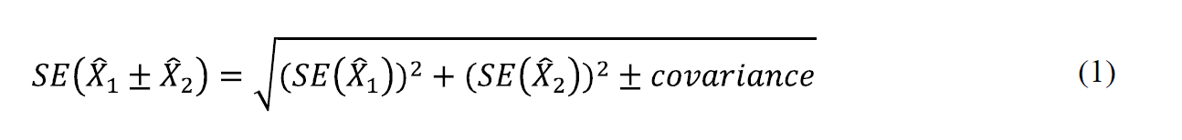
The covariance measures the interactions between two estimates. Currently the covariance terms are not available. Data users should use the approximation:
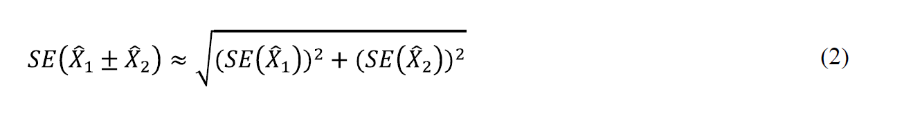
However, this method will underestimate or overestimate the standard error if the two estimates interact in either a positive or negative way. The approximation formula (2) can be expanded to more than two estimates by adding in the individual standard errors squared inside the radical. As the number of estimates involved in the sum or difference increases, the results of formula (2) become increasingly different from the standard error derived directly from the ACS microdata. Care should be taken to work with the fewest number of estimates as possible. If there are estimates involved in the sum that are controlled in the weighting then the approximate standard error can be increasingly different.
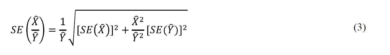
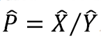 , then the standard error of this proportion is approximated as:
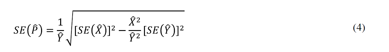
If Q = 100% x P (P is the proportion and Q is its corresponding percent), then SE(Q) = 100% x SE(P).
Note the difference between the formulas to approximate the standard error for proportions (4) and ratios (3) - the plus sign in the previous formula has been replaced with a minus sign. If the value under the radical is negative, use the ratio standard error formula above, instead.
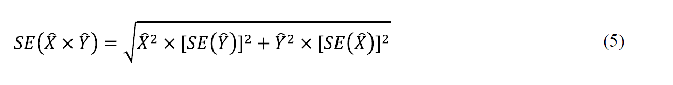
Comparing 1-Year Period Estimates with Overlapping 3-Year Period Estimates It should be noted that the 1-year and 3-year estimates represent period estimates. Due to the difficulty in interpreting the 'difference' in period estimates of different lengths, the Census Bureau currently discourages users from making such comparisons. The standard error of this difference is approximated as:
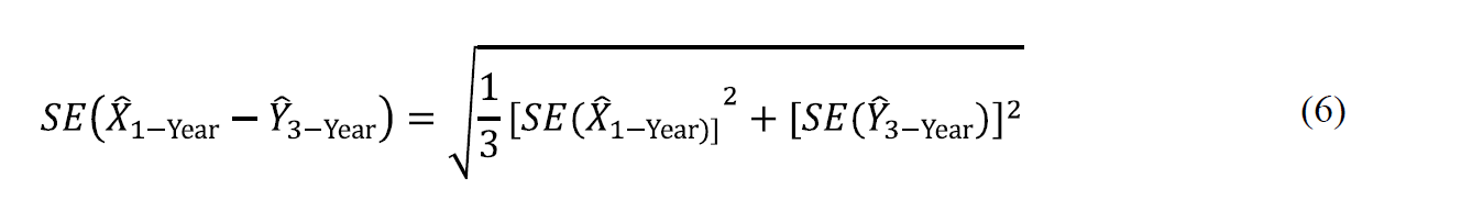
Comparing 1-Year Period Estimates with Overlapping 5-Year Period Estimates It should be noted that the 1-year and 5-year estimates represent period estimates. Due to the difficulty in interpreting the 'difference' in period estimates of different lengths, the Census Bureau currently discourages users from making such comparisons. The standard error of this difference is approximated as:
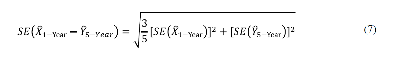
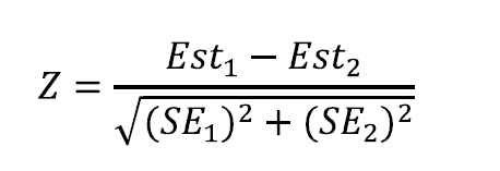
If Z > 1.645 or Z < -1.645, then the difference can be said to be statistically significant at the 90 percent confidence level.
Any estimate can be compared to an ACS estimate using this method, including other ACS estimates from the current year, the ACS estimate for the same characteristic and geographic area but from a previous year, Census 2000 100 percent counts and long form estimates, estimates from other Census Bureau surveys, and estimates from other sources.
Not all estimates have sampling error - Census 2000 100 percent counts do not, for example, although Census 2000 long form estimates do - but they should be used if they exist to give the most accurate result of the test. Users are also cautioned to not rely on looking at whether confidence intervals for two estimates overlap or not to determine statistical significance, because there are circumstances where that method will not give the correct test result. If two confidence intervals do not overlap, then the estimates will be significantly different (i.e. the significance test will always agree). However, if two confidence intervals do overlap, then the estimates may or may not be significantly different.
The Z calculation above is recommended in all cases.2
The ACS Accuracy of the Data document in 2005 used a Z statistic of +/-1.65. Data users should use +/-1.65 for estimates published in 2005 or earlier.Here is a simple example of why it is not recommended to use the overlapping confidence bounds rule of thumb as a substitute for a statistical test.
Let: X1 = 5.0 with SE1 = 0.2 and X2 = 6.0 with SE2 = 0.5.
The Upper Bound for X1 = 5.0 + 0.2 * 1.645 = 5.3 while
the Lower Bound for X2 = 6.0 - 0.5 * 1.645 = 5.2.
The confidence bounds overlap, so, the rule of thumb would indicate that the estimates are not significantly different at the 90% level. However, if we apply the statistical significance test we obtain:
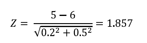
Z = 1.857 > 1.645 which means that the difference is significant (at the 90% level).All statistical testing in ACS data products is based on the 90 percent confidence level.
Users should understand that all testing was done using unrounded estimates and standard errors, and it may not be possible to replicate test results using the rounded estimates and margins of error as published.
Example 1 - Calculating the Standard Error from the Confidence Interval
The estimated number of males, never married is 42,157,997 from summary table B12001 for the United States for 2009.
The margin of error is 101,091.
Standard Error = Margin of Error / 1.645
Calculating the standard error using the margin of error, we have:
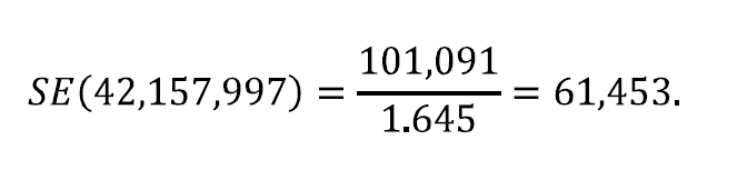
Example 2 - Calculating the Standard Error of a Sum or a Difference
We are interested in the number of people who have never been married.
From Example 1, we know the number of males, never married is 42,157,997. From summary table B12001 we have the number of females, never married is 35,852,821 with a margin of error of 87,607. So, the estimated number of people who have never been married is 42,157,997 + 35,852,821 = 78,010,818.
To calculate the approximate standard error of this sum, we need the standard errors of the two estimates in the sum. We have the standard error for the number of males never married from example 1 as 61,453. The standard error for the number of females never married is calculated using the margin of error:
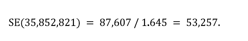
So using formula (2) for the approximate standard error of a sum or difference we have:
Caution: This method will underestimate or overestimate the standard error if the two estimates interact in either a positive or negative way. To calculate the lower and upper bounds of the 90 percent confidence interval around 78,010,818 using the standard error, simply multiply 81,319 by 1.645, then add and subtract the product from 78,010,818. Thus the 90 percent confidence interval for this estimate is
[78,010,818 - 1.645(81,319)] to [78,010,818 + 1.645(81,319)] or 77,877,048 to 78,144,588.
Example 3 - Calculating the Standard Error of a Proportion/Percent
We are interested in the percentage of females who have never been married to the number of people who have never been married. The number of females, never married is 35,852,821 and the number of people who have never been married is 78,010,818. To calculate the approximate standard error of this percent, we need the standard errors of the two estimates in the percent. We have the approximate standard error for the number of females never married from example 2 as 53,257 and the approximate standard error for the number of people never married calculated from example 2 as 81,319. The estimate is

So, using formula (4) for the approximate standard error of a proportion or percent, we have:
To calculate the lower and upper bounds of the 90 percent confidence interval around 45.96 using the standard error, simply multiply 0.05 by 1.645, then add and subtract the product from 45.96. Thus the 90 percent confidence interval for this estimate is
[45.96 - 1.645(0.05)] to [45.96 + 1.645(0.05)], or 45.88% to 46.04%.
Example 4 - Calculating the Standard Error of a Ratio
Now, let us calculate the estimate of the ratio of the number of unmarried males to the number of unmarried females and its approximate standard error. From the above examples, the estimate for the number of unmarried men is 42,157,997 with a standard error of 61,453, and the estimate for the number of unmarried women is 35,852,821 with a standard error of 53,257. The estimate of the ratio is 42,157,997 / 35,852,821 = 1.176. Using formula (3) for the approximate standard error of this ratio we have:
The 90 percent margin of error for this estimate would be 0.00245 multiplied by 1.645, or about 0.004. The 90 percent lower and upper 90 percent confidence bounds would then be
[1.176 - 0.004] to [1.176 + 0.004], or 1.172 and 1.180.
Example 5 - Calculating the Standard Error of a Product
We are interested in the number of 1-unit detached owner-occupied housing units. The number of owner-occupied housing units is 74,843,004 with a margin of error of 217,682 from subject table S2504 for 2009, and the percent of 1-unit detached owner-occupied housing units is 81.8% (0.818) with a margin of error of 0.1 (0.001). So the number of 1-unit detached owner-occupied housing units is
74,843,004 * 0.818 = 61,221,577.
Calculating the standard error for the estimates using the margin of error we have:
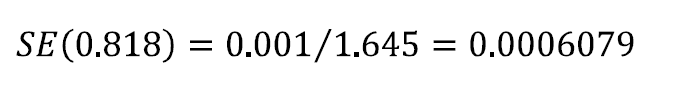
and

To calculate the lower and upper bounds of the 90 percent confidence interval around 61,221,577 using the standard error, simply multiply 117,418 by 1.645, then add and subtract the product from 61,221,577. Thus the 90 percent confidence interval for this estimate is
[61,221,577 - 1.645(117,418)] to [61,221,577 + 1.645(117,418)] or 61,028,424 to 61,414,730.
- Coverage Error - It is possible for some sample housing units or persons to be missed entirely by the survey (undercoverage), but it is also possible for some sample housing units and persons to be counted more than once (overcoverage). Both the undercoverage and overcoverage of persons and housing units can introduce biases into the data, increase respondent burden and survey costs.
A major way to avoid coverage error in a survey is to ensure that its sampling frame, for ACS an address list in each state, is as complete and accurate as possible. The source of addresses for the ACS is the MAF, which was created by combining the Delivery Sequence File of the United States Postal Service and the address list for Census 2000. An attempt is made to assign all appropriate geographic codes to each MAF address via an automated procedure using the Census Bureau TIGER (Topologically Integrated Geographic Encoding and Referencing) files. A manual coding operation based in the appropriate regional offices is attempted for addresses which could not be automatically coded. The MAF was used as the source of addresses for selecting sample housing units and mailing questionnaires. TIGER produced the location maps for CAPI assignments. Sometimes the MAF has an address that is the duplicate of another address already on the MAF. This could occur when there is a slight difference in the address such as 123 Main Street versus 123 Maine Street.In the CATI and CAPI nonresponse follow-up phases, efforts were made to minimize the chances that housing units that were not part of the sample were interviewed in place of units in sample by mistake. If a CATI interviewer called a mail nonresponse case and was not able to reach the exact address, no interview was conducted and the case was eligible for CAPI. During CAPI follow-up, the interviewer had to locate the exact address for each sample housing unit. If the interviewer could not locate the exact sample unit in a multi-unit structure, or found a different number of units than expected, the interviewers were instructed to list the units in the building and follow a specific procedure to select a replacement sample unit. Person overcoverage can occur when an individual is included as a member of a housing unit but does not meet ACS residency rules. Coverage rates give a measure of undercoverage or overcoverage of persons or housing units in a given geographic area. Rates below 100 percent indicate undercoverage, while rates above 100 percent indicate overcoverage. Coverage rates are released concurrent with the release of estimates on American FactFinder in the B98 series of detailed tables. Further information about ACS coverage rates may be found at http://www.census.gov/acs/www/methodology/sample_size_and_data_quality/.
- Nonresponse Error - Survey nonresponse is a well-known source of nonsampling error. There are two types of nonresponse error - unit nonresponse and item nonresponse. Nonresponse errors affect survey estimates to varying levels depending on amount of nonresponse and the extent to which nonrespondents differ from respondents on the characteristics measured by the survey. The exact amount of nonresponse error or bias on an estimate is almost never known. Therefore, survey researchers generally rely on proxy measures, such as the nonresponse rate, to indicate the potential for nonresponse error.
- Unit Nonresponse - Unit nonresponse is the failure to obtain data from housing units in the sample. Unit nonresponse may occur because households are unwilling or unable to participate, or because an interviewer is unable to make contact with a housing unit. Unit nonresponse is problematic when there are systematic or variable differences between interviewed and noninterviewed housing units on the characteristics measured by the survey. Nonresponse bias is introduced into an estimate when differences are systematic, while nonresponse error for an estimate evolves from variable differences between interviewed and noninterviewed households.
The ACS makes every effort to minimize unit nonresponse, and thus, the potential for nonresponse error. First, the ACS used a combination of mail, CATI, and CAPI data collection modes to maximize response. The mail phase included a series of three to four mailings to encourage housing units to return the questionnaire. Subsequently, mail nonrespondents (for which phone numbers are available) were contacted by CATI for an interview. Finally, a subsample of the mail and telephone nonrespondents was contacted by personal visit to attempt an interview. Combined, these three efforts resulted in a very high overall response rate for the ACS.ACS response rates measure the percent of units with a completed interview. The higher the response rate, and consequently the lower the nonresponse rate, the less chance estimates may be affected by nonresponse bias. Response and nonresponse rates, as well as rates for specific types of nonresponse, are released concurrent with the release of estimates on American FactFinder in the B98 series of detailed tables. Further information about response and nonresponse rates may be found at http://www.census.gov/acs/www/methodology/sample_size_and_data_quality/.
- Item Nonresponse - Nonresponse to particular questions on the survey questionnaire and instrument allows for the introduction of error or bias into the data, since the characteristics of the nonrespondents have not been observed and may differ from those reported by respondents. As a result, any imputation procedure using respondent data may not completely reflect this difference either at the elemental level (individual person or housing unit) or on average.
Some protection against the introduction of large errors or biases is afforded by minimizing nonresponse. In the ACS, item nonresponse for the CATI and CAPI operations was minimized by the requirement that the automated instrument receive a response to each question before the next one could be asked. Questionnaires returned by mail were edited for completeness and acceptability. They were reviewed by computer for content omissions and population coverage. If necessary, a telephone follow-up was made to obtain missing information. Potential coverage errors were included in this follow-up. Allocation tables provide the weighted estimate of persons or housing units for which a value was imputed, as well as the total estimate of persons or housing units that were eligible to answer the question. The smaller the number of imputed responses, the lower the chance that the item nonresponse is contributing a bias to the estimates. Allocation tables are released concurrent with the release of estimates on American Factfinder in the B99 series of detailed tables with the overall allocation rates across all person and housing unit characteristics in the B98 series of detailed tables. Additional information on item nonresponse and allocations can be found at
- Measurement and Processing Error - The person completing the questionnaire or responding to the questions posed by an interviewer could serve as a source of error, although the questions were cognitively tested for phrasing and detailed instructions for completing the questionnaire were provided to each household.
- Interviewer monitoring - The interviewer may misinterpret or otherwise incorrectly enter information given by a respondent; may fail to collect some of the information for a person or household; or may collect data for households that were not designated as part of the sample. To control these problems, the work of interviewers was monitored carefully. Field staff were prepared for their tasks by using specially developed training packages that included hands-on experience in using survey materials. A sample of the households interviewed by CAPI interviewers was reinterviewed to control for the possibility that interviewers may have fabricated data.
- Processing Error - The many phases involved in processing the survey data represent potential sources for the introduction of nonsampling error. The processing of the survey questionnaires includes the keying of data from completed questionnaires, automated clerical review, follow-up by telephone, manual coding of write-in responses, and automated data processing. The various field, coding and computer operations undergo a number of quality control checks to insure their accurate application.
- Content Editing - After data collection was completed, any remaining incomplete or inconsistent information was imputed during the final content edit of the collected data. Imputations, or computer assignments of acceptable codes in place of unacceptable entries or blanks, were needed most often when an entry for a given item was missing or when the information reported for a person or housing unit on that item was inconsistent with other information for that same person or housing unit. As in other surveys and previous censuses, the general procedure for changing unacceptable entries was to allocate an entry for a person or housing unit that was consistent with entries for persons or housing units with similar characteristics. Imputing acceptable values in place of blanks or unacceptable entries enhances the usefulness of the data.
Table A: 2009 Estimates of Males with Income Below Poverty from table C17001: Poverty Status in the Past 12 Months by Sex by Age
| Characteristic | Wyoming | PUMA 00100 | PUMA 00200 | PUMA 00300 | PUMA 00400 |
|---|---|---|---|---|---|
| Male | 23,001 (3,309) | 5,264 (1,624) | 6,508 (1,395) | 4,364 (1,026) | 6,865 (1,909) |
| Under 18 Years Old | 8,479 (1,874) | 2,041 (920) | 2,222 (778) | 1,999 (750) | 2,217 (1,192) |
| 18 to 64 Years Old | 12,976 (2,076) | 3,004 (1,049) | 3,725 (935) | 2,050 (635) | 4,197 (1,134) |
| 65 Years and Older | 1,546 (500) | 219 (237) | 561 (286) | 315 (173) | 451 (302) |
2009 American FactFinder
The first way is to sum the three age groups for Wyoming:
Estimate(Male) = 8,479 + 12,976 + 1,546 = 23,001.
The first approximation for the standard error in this case gives us:
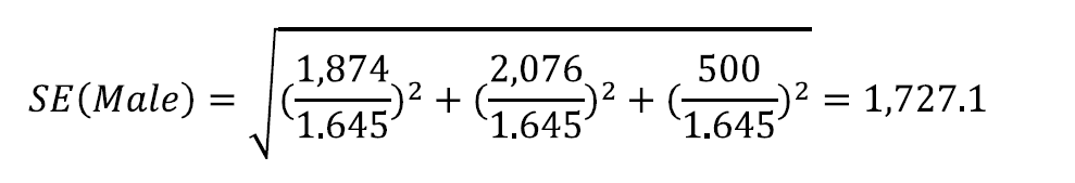
A second way is to sum the four PUMA estimates for Male to obtain: Estimate(Male) = 5,264 + 6,508 + 4,364 + 6,865 = 23,001 as before. The second approximation for the standard error yields:
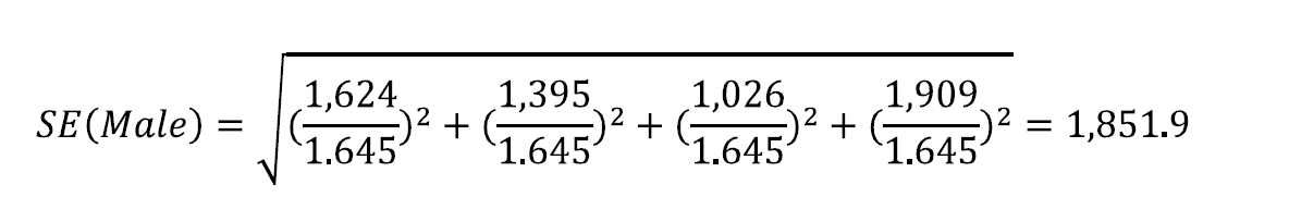
Finally, we can sum up all three age groups for all four PUMAs to obtain an estimate based on a total of twelve estimates:
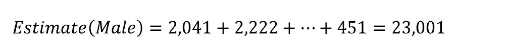
And the third approximated standard error is
However, we do know that the standard error using the published MOE is 3,309 /1.645 = 2,011.6. In this instance, all of the approximations under-estimate the published standard error and should be used with caution. B. Suppose we wish to estimate the total number of males at the national level using age and citizenship status. The relevant data from table B05003 is displayed in table B below.
Table B: 2009 Estimates of males from B05003: Sex by Age by Citizenship Status
| Characteristic | Estimate | MOE |
|---|---|---|
| Male | 151,375,321 | 27,279 |
| Under 18 Years | 38,146,514 | 24,365 |
| Native | 36,747,407 | 31,397 |
| Foreign Born | 1,399,107 | 20,177 |
| Naturalized U.S. Citizen | 268,445 | 10,289 |
| Not a U.S. Citizen | 1,130,662 | 20,228 |
| 18 Years and Older | 113,228,807 | 23,525 |
| Native | 95,384,433 | 70,210 |
| Foreign Born | 17,844,374 | 59,750 |
| Naturalized U.S. Citizen | 7,507,308 | 39,658 |
| Not a U.S. Citizen | 10,337,066 | 65,533 |
2009 American FactFinder
The estimate and its MOE are actually published. However, if they were not available in the tables, one way of obtaining them would be to add together the number of males under 18 and over 18 to get:

And the first approximated standard error is
Another way would be to add up the estimates for the three subcategories (Native, and the two subcategories for Foreign Born: Naturalized U.S. Citizen, and Not a U.S. Citizen), for males under and over 18 years of age. From these six estimates we obtain:
With a second approximated standard error of:
We do know that the standard error using the published margin of error is 27,279 / 1.645 = 16,583.0. With a quick glance, we can see that the ratio of the standard error of the first method to the published-based standard error yields 1.24; an over-estimate of roughly 24%, whereas the second method yields a ratio of 4.07 or an over-estimate of 307%. This is an example of what could happen to the approximate SE when the sum involves a controlled estimate. In this case, it is sex by age.C. Suppose we are interested in the total number of people aged 65 or older and its standard error. Table C shows some of the estimates for the national level from table B01001 (the estimates in gray were derived for the purpose of this example only).
Table C: Some Estimates from AFF Table B01001: Sex by Age for 2009
| Age Category | Estimate, Male | MOE, Male | Estimate, Female | MOE, Female | Total | Estimated MOE, Total |
|---|---|---|---|---|---|---|
| 65 and 66 years old | 2,492,871 | 20,194 | 2,803,516 | 23,327 | 5,296,387 | 30,854 |
| 67 to 69 years old | 3,029,709 | 18,280 | 3,483,447 | 24,287 | 6,513,225 | 30,398 |
| 70 to 74 years old | 4,088,428 | 21,588 | 4,927,666 | 26,867 | 9,016,094 | 34,466 |
| 75 to 79 years old | 3,168,175 | 19,097 | 4,204,401 | 23,024 | 7,372,576 | 29,913 |
| 80 to 84 years old | 2,258,021 | 17,716 | 3,538,869 | 25,423 | 5,796,890 | 30,987 |
| 85 years and older | 1,743,971 | 17,991 | 3,767,574 | 19,294 | 5,511,545 | 26,381 |
| Total | 16,781,175 | NA | 22,725,473 | NA | 39,506,648 | 74,932 |
To begin we find the total number of people aged 65 and over by simply adding the totals for males and females to get 16,781,175 + 22,725,542 = 39,506,717. One way we could use is summing males and female for each age category and then using their MOEs to approximate the standard error for the total number of people over 65.
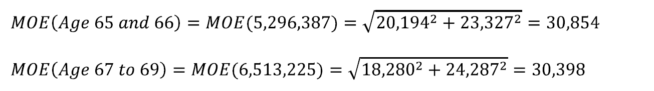
... etc ...
Now, we calculate for the number of people aged 65 or older to be 39,506,648 using the six derived estimates and approximate the standard error:
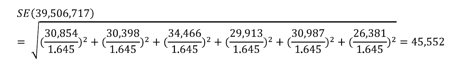
For this example the estimate and its MOE are published in table B09017. The total number of people aged 65 or older is 39,506,648 with a margin of error of 20,689. Therefore the published-based standard error is:
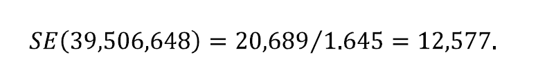
The approximated standard error, using six derived age group estimates, yields an approximated standard error roughly 3.6 times larger than the published-based standard error. As a note, there are two additional ways to approximate the standard error of people aged 65 and over in addition to the way used above. The first is to find the published MOEs for the males age 65 and older and of females aged 65 and older separately and then combine to find the approximate standard error for the total. The second is to use all twelve of the published estimates together, that is, all estimates from the male age categories and female age categories, to create the SE for people aged 65 and older. However, in this particular example, the results from all three ways are the same. So no matter which way you use, you will obtain the same approximation for the SE. This is different from the results seen in example A. D. For an alternative to approximating the standard error for people 65 years and older seen in part C, we could find the estimate and its SE by summing all of the estimate for the ages less than 65 years old and subtracting them from the estimate for the total population. Due to the large number of estimates, Table D does not show all of the age groups. In addition, the estimates in part of the table shaded gray were derived for the purposes of this example only and cannot be found in base table B01001.
Table D: Some Estimates from AFF Table B01001: Sex by Age for 2009:
| Age Category | Estimate, Male | MOE, Male | Estimate, Female | MOE, Female | Total | Estimated MOE, Total |
|---|---|---|---|---|---|---|
| Total Population | 151,375,321 | 27,279 | 155,631,235 | 27,280 | 307,006,556 | 38,579 |
| Under 5 years | 10,853,263 | 15,661 | 10,355,944 | 14,707 | 21,209,207 | 21,484 |
| 5 to 9 years old | 10,273,948 | 43,555 | 9,850,065 | 42,194 | 20,124,013 | 60,641 |
| 10 to 14 years old | 10,532,166 | 40,051 | 9,985,327 | 39,921 | 20,517,493 | 56,549 |
| ... | ... | ... | ... | ... | ||
| 62 to 64 years old | 4,282,178 | 25,636 | 4,669,376 | 28,769 | 8,951,554 | 38,534 |
| Total for Age 0 to 64 years old | 134,594,146 | 117,166 | 132,905,762 | 117,637 | 267,499,908 | 166,031 |
| Total for Age 65 years and older | 16,781,175 | 120,300 | 22,725,473 | 120,758 | 39,506,648 | 170,454 |
An estimate for the number of people age 65 and older is equal to the total population minus the population between the ages of zero and 64 years old: Number of people aged 65 and older: 307,006,556 - 267,499,908 = 39,506,648. The way to approximate the SE is the same as in part C. First we will sum male and female estimates across each age category and then approximate the MOEs. We will use that information to approximate the standard error for our estimate of interest:
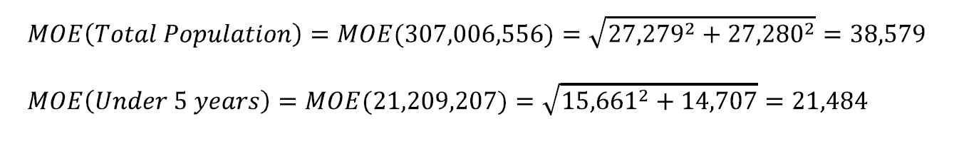
... etc ...
And the SE for the total number of people aged 65 and older is:
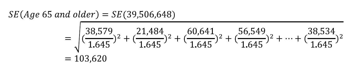
Again, as in Example C, the estimate and its MOE are we published in B09017. The total number of people aged 65 or older is 39,506,648 with a margin of error of 20,689. Therefore the standard error is:
SE(39,506,648) = 20,689 / 1.645 = 12,577.
The approximated standard error using the thirteen derived age group estimates yields a standard error roughly 8.2 times larger than the actual SE. Data users can mitigate the problems shown in examples A through D to some extent by utilizing a collapsed version of a detailed table (if it is available) which will reduce the number of estimates used in the approximation. These issues may also be avoided by creating estimates and SEs using the Public Use Microdata Sample (PUMS) or by requesting a custom tabulation, a fee-based service offered under certain conditions by the Census Bureau. More information regarding custom tabulations may be found at http://www.census.gov/acs/www/data_documentation/custom_tabulations/
- Mailout/Mailback
- Computer Assisted Telephone Interview (CATI)
- Computer Assisted Personal Interview (CAPI)
The general timing of data collection is:
Month 1: Addresses in sample that are determined to be mailable are sent a questionnaire via the U.S. Postal Service.
Month 2: All mail non-responding addresses with an available phone number are sent to CATI.
Month 3: A sample of mail non-responses without a phone number, CATI non-responses, and unmailable addresses are selected and sent to CAPI.
Note that mail responses are accepted during all three months of data collection.
Group Quarters data collection spans six weeks, except for Federal prisons, where the data collection time period is four months. All Federal prisons are assigned to September with a four month data collection window.
The Main sample is selected during the summer preceding the sample year. Approximately 99 percent of the sample is selected at this time. Each address in sample is randomly assigned to one of the 12 months of the sample year. Supplemental sampling occurs in January/February of the sample year and accounts for approximately 1 percent of the overall first-phase sample. The Supplemental sample is allocated to the last nine months of the sample year. A sub-sample of non-responding addresses and of any addresses deemed unmailable is selected for the CAPI data collection mode. Several of the steps used to select the first-phase sample are common to both Main and Supplemental sampling. The descriptions of the steps included in the first-phase sample selection below indicate which are common to both and which are unique to either Main or Supplemental sampling.
1. First-phase Sample Selection
- First-stage sampling (performed during both Main and Supplemental sampling) - First stage sampling defines the universe for the second stage of sampling through two steps. First, all addresses that were in a first-phase sample within the past four years are excluded from eligibility. This ensures that no address is in sample more than once in any five-year period. The second step is to select a 20 percent systematic sample of 'new' units, i.e. those units that have never appeared on a previous MAF extract. Each new address is systematically assigned to either the current year or to one of four back-samples. This procedure maintains five equal partitions of the universe.
- Assignment of blocks to a second-stage sampling stratum (performed during Main sampling only) - Second-stage sampling uses five sampling strata in PR. The stratum level rates used in second-stage sampling account for the first-stage selection probabilities. These rates are applied at a block level to addresses in PR by calculating a measure of size for Municipios.
The measure of size is an estimate of the number of occupied HUs in the Municipio. This is calculated by multiplying the number of PRCS addresses by the occupancy rate from Census 2000 at the block level. A measure of size for each Census Tract is also calculated in the same manner. Each block is then assigned the smallest measure of size from the set of all entities of which it is a part.
The second-stage sampling strata and the overall first-phase sampling rates are shown in Table 1 below.
- Calculation of the second-stage sampling rates (performed during Main sampling only) - The overall first-phase sampling rates given in Table 1 are calculated using the distribution of PRCS valid addresses by second-stage sampling stratum in such a way as to yield an overall target sample size for the year of approximately 36,000. These rates also account for expected growth of the HU inventory between Main and Supplemental of roughly 1 percent. The first-phase rates are adjusted for the first-stage sample to yield the second-stage selection probabilities.
- Second-stage sample selection (performed in Main and Supplemental) - After each block is assigned to a second-stage sampling stratum, a systematic sample of addresses is selected from the second-stage universe (first- stage sample) within each municipio.
- Sample Month Assignment (performed in Main and Supplemental) - After the second stage of sampling, all sample addresses are randomly assigned to a sample month. Addresses selected during Main sampling are allocated to each of the 12 months. Addresses selected during Supplemental sampling are assigned to the months of April-December.
| Sampling Rate Category | Sampling Rates |
|---|---|
| Blocks in smallest Municipios (MOS1 < 200) | 10.0% |
| Blocks in smaller Municipios (200 ≤ MOS < 800) | 8.04% |
| Blocks in small Municipios (800 ≤ MOS ≤ 1200) | 4.02% |
| Blocks in large Municipios (MOS >1200, TRACTMOS2≥ 2000) | 2.01% |
| All other blocks (MOS >1200, TRACTMOS < 2000) | 2.68% |
Footnote:
1MOS = Measure of size.
2TRACTMOS = Census Tract measure of size.
2. Second-phase Sample Selection - Subsampling the Unmailable and Non-Responding Addresses
All addresses determined to be unmailable are subsampled for the CAPI phase of data collection at a rate of 2-in-3. Unmailable addresses do not go to the CATI phase of data collection. Subsequent to CATI, all addresses for which no response has been obtained prior to CAPI are subsampled based on the expected rate of completed interviews at the tract level using the rates shown in Table 2.
| Address Characteristics | CAPI Subsampling Rate |
|---|---|
| Unmailable addresses | 66.7% |
| Mailable addresses | 50% |
1Note that all references to the small GQ stratum include both small GQs and GQs closed on Census day.
1. First-phase Sample Selection for Small GQ Stratum
- First-stage sampling - Small GQs are only eligible to be selected for the PRCS once every five years. To accomplish this, the first stage sampling procedure systematically assigned all small GQs to one of five partitions of the universe. Each partition was assigned to a particular year (2009-2012) and the one assigned to 2009 became the first stage sample. In future years, each new GQ will be systematically assigned to one of the five samples. These samples are rotated over five year periods and become the universe for selecting the second stage sample.
- Second-stage sampling - A simple 1-in-8 systematic sample of the GQs in the first stage sample is selected. Regardless of their actual size, all GQs in the small stratum have the same probability of selection. Since the first stage sample is 20% of the universe, this yields the targeted sampling rate of 2.5%.
2. Sample Selection for the Large GQ Stratum
Unlike housing unit address sampling and the small GQ sample selection, the large GQ sampling procedure has no first-stage in which sampling units are randomly assigned to one of five years. All large GQs are eligible for sampling each year. The large GQ samples are selected using a two-phase design.
- First-phase Sampling - In the large GQ stratum, GQ hits are selected using a systematic PPS (probability proportional to size) sample, with a target sampling rate of 2.5%. A hit refers to a grouping of 10 expected interviews. GQs are selected with probability proportional to its most current count of persons or capacity. For stratification, and for sampling the large GQs, a GQ measure of size (GQMOS) is computed, where GQMOS is the expected population of the GQ divided by 10. This reflects that the GQ data is collected in groups of 10 GQ persons. People are selected in hits of 10 in a systematic sample of 1-in-40 hits. All GQs in this stratum are eligible for sampling every year, regardless of their sample status in previous years. For large GQs, hits can be selected multiple times in the sample year. For most GQ types, the hits are randomly assigned throughout the year. Some GQs may have multiple hits with the same sample date if more than 12 hits are selected from the GQ. In these cases, the person sample within that month is unduplicated.
3. Sample Month AssignmentIn order to assign a panel month to each hit, all of the GQ samples from Puerto Rico are combined and sorted by small/large stratum and second-phase order of selection. Consecutive samples are assigned to the twelve panel months in a predetermined order, starting with a randomly determined month, except for Federal prisons. Correctional facilities have their sample clustered. All Federal prisons hits are assigned to the September panel. In non-Federal correctional facilities, all hits for a given GQ are assigned to the same panel month. However, unlike Federal prisons, the hits in state and local correctional facilities are assigned to randomly selected panels spread throughout the year.
4. Second Phase Sample: Selection of Persons in Small and Large GQs
Small GQs in the second phase sampling are 'take all,' i.e., every person in the selected GQ is eligible to receive a questionnaire. If the actual number of persons in the GQ exceeds 15, a field subsampling operation is performed to reduce the total number of sample persons interviewed at the GQ to 10. If the actual number of persons in the GQ is 10 or fewer, then the group size will be less than 10.
For each hit in the large GQs, the automated instrument uses the population count at the time of the visit and selects a subsample of 10 people from the roster. The people in this subsample receive the questionnaire.
The weighting is conducted in two main operations: a group quarters person weighting operation which assigns weights to persons in group quarters, and a household person weighting operation which assigns weights both to housing units and to persons within housing units. The group quarters person weighting is conducted first and the household person weighting second. The household person weighting is dependent on the group quarters person weighting because estimates for total population, which include both group quarters and household population, are controlled to the Census Bureau' s official 2009 total resident population estimates.
The major type groups used are:
Table 3: Population Estimates Program Major GQ Type Groups
| Major GQ Type Group | Definition | Institutional / Non-Institutional |
|---|---|---|
| 1 | Correctional Institutions | Institutional |
| 2 | Juvenile Detention Facilities | Institutional |
| 3 | Nursing Homes | Institutional |
| 4 | Other Long-Term Care Facilities | Institutional |
| 5 | College Dormitories | Non-Institutional |
| 6 | Military Facilities | Non-Institutional |
| 7 | Other Non-Institutional Facilities | Non-Institutional |
The procedure used to assign the weights to the GQ persons is performed independently within the commonwealth of Puerto Rico. The steps to assign the weights to the GQ persons are as follows:
- Base Weight-The initial base weight after the first phase of sampling is the inverse of its first-phase sampling rate, which is equal to 40 for all sample cases in 2009. This initial base weight is then adjusted for the second-phase sampling that occurs at the time of interview.
- Non-Interview Factor-This factor adjusts the weight of all responding GQ persons to account for the non-responding GQ persons including those persons contained in whole non-responding GQs. The non-interview factor is computed and assigned using the following groups:
Major GQ Type Group x Municipio
- GQ Person Post-stratification Factor-This factor adjusts the GQ person weights so that the weighted sample counts equal independent population estimates from the Population Estimates Program by Major Type Group for the commonwealth of Puerto Rico. Because of collapsing of groups in applying this factor, only total GQ population is assured of agreeing with the Census Bureau' s official 2009 population estimates. The GQ person post-stratification factor is computed and assigned using the following groups:
Major GQ Type Group
- Rounding-The final GQ person weight is rounded to an integer. Rounding is performed so that the sum of the rounded weights is within one person of the sum of the unrounded weights for any of the groups listed below:
Major GQ Type Group
Major GQ Type Group x Municipio
- Percent in poverty
- Percent renting
- Percent in rural areas
- Race/ethnicity, age, and sex distribution
- Distance between the centroids of the municipios
- Core-based Statistical Area status:
Each weighting area is also required to meet a threshold of 400 expected person interviews in the 2009 PRCS. The process also tries to preserve as many municipios that met the threshold to form their own weighting areas. In total, there are 55 weighting areas formed from the 78 municipios in Puerto Rico. The estimation procedure used to assign the weights is then performed independently within each of the PRCS weighting areas.
1.Initial Housing Unit Weighting Factors.
This process produces the following factors:
- Base Weight (BW)-This initial weight is assigned to every housing unit as the inverse of its block' s sampling rate.
- CAPI Subsampling Factor (SSF)-The weights of the CAPI cases are adjusted to reflect the results of CAPI subsampling. This factor is assigned to each record as follows:
Selected in CAPI subsampling: SSF = 2.0
Not selected in CAPI subsampling: SSF = 0.0
Not a CAPI case: SSF = 1.0
Some sample addresses are unmailable. A two-thirds sample of these is sent directly to CAPI and for these cases SSF = 1.5.
- Variation in Monthly Response by Mode (VMS)-This factor makes the total weight of the Mail, CATI, and CAPI records to be tabulated in a month equal to the total base weight of all cases originally mailed for that month. For all cases, VMS is computed and assigned based on the following groups:
Weighting Area x Month
- Noninterview Factor (NIF)-This factor adjusts the weight of all responding occupied housing units to account for nonresponding housing units. The factor is computed in two stages. The first factor, NIF1, is a ratio adjustment that is computed and assigned to occupied housings units based on the following groups:
Weighting Area x Building Type x Tract
A second factor, NIF2, is a ratio adjustment that is computed and assigned to occupied housing units based on the following groups:
Weighting Area x Building Type x Month
NIF is then computed by applying NIF1 and NIF2 for each occupied housing unit. Vacant housing units are assigned a value of NIF = 1.0. Nonresponding housing units are now assigned a weight of 0.0.
- Noninterview Factor-Mode (NIFM)-This factor adjusts the weight of the responding CAPI occupied housing units to account for CAPI nonrespondents. It is computed as if NIF had not already been assigned to every occupied housing unit record. This factor is not used directly but rather as part of computing the next factor, the Mode Bias Factor.
NIFM is computed and assigned to occupied CAPI housing units based on the following groups: Weighting Area x Building Type (single or multi unit) x Month Vacant housing units or non-CAPI (mail and CATI) housing units receive a value of NIFM = 1.0.
- Mode Bias Factor (MBF)-This factor makes the total weight of the housing units in the groups below the same as if NIFM had been used instead of NIF. MBF is computed and assigned to occupied housing units based on the following groups:
Weighting Area x Tenure (owner or renter) x Month x Marital Status of the Householder (married/widowed or single)
Vacant housing units receive a value of MBF = 1.0. MBF is applied to the weights computed through NIF.
2.Person Weighting Factors-Initially the person weight of each person in an occupied housing unit is the product of the weighting factors of their associated housing unit (BW x ... x MBF). At this point everyone in the household has the same weight. The person weighting is done in a series of three steps which are repeated until a stopping criterion is met. These three steps form a raking ratio or raking process. These person weights are individually adjusted for each person as described below.
The three steps are as follows:
- Municipio Controls Raking Factor (SUBEQRF) - This factor is applied to individuals based on their geography. It adjusts the person weights so that the weighted sample counts equal independent population estimates of total population for the municipio. For those municipios which are their own weighting area, this adjustment factor will be 1.0. Because of later adjustments to the person weights, total population is not assured of agreeing exactly with the official 2009 population estimates for municipios which are not their own weighting area.
- Spouse Equalization/Householder Equalization Raking Factor (SPHHEQRF)-This factor is applied to individuals based on the combination of their status of being in a married-couple or unmarried-partner household and whether they are the householder. All persons are assigned to one of four groups:
- Householder in a married-couple or unmarried-partner household
- Spouse or unmarried partner in a married-couple or unmarried-partner household (non-householder)
- Other householder
- Other non-householder
The weights of persons in the first two groups are adjusted so that their sums are each equal to the total estimate of married-couple or unmarried-partner households using the housing unit weight (BW x ... x HPF). At the same time the weights of persons in the first and third groups are adjusted so that their sum is equal to the total estimate of occupied housing units using the housing unit weight (BW x ... x HPF). The goal of this step is to produce more consistent estimates of spouses or unmarried partners and married-couple and unmarried-partner households while simultaneously producing more consistent estimates of householders, occupied housing units, and households.
- Demographic Raking Factor (DEMORF)-This factor is applied to individuals based on their age and sex in Puerto Rico (note that there are 13 Age groupings). It adjusts the person weights so that the weighted sample counts equal the independent population estimates by age and sex at the weighting area level. Because of collapsing of groups in applying this factor, only the total population is assured of agreeing with the official 2009 population estimates at the weighting area level.
These three steps are repeated several times until the estimates for Puerto Rico achieve their optimal consistency with regard to the spouse and householder equalization. The Person Post-Stratification Factor (PPSF) is then equal to the product (SUBEQRF x SPHHEQRF x DEMORF) from all of iterations of these three adjustments. The unrounded person weight is then the equal to the product of PPSF times the housing unit weight (BW x ... x MBF x PPSF). 3.Rounding-The final product of all person weights (BW x ...MBF x PPSF) is rounded to an integer. Rounding is performed so that the sum of the rounded weights is within one person of the sum of the unrounded weights for any of the groups listed below:
Municipio
Municipio x Sex
Municipio x Sex x Age
Municipio x Sex x Age x Tract
Municipio x Sex x Age x Tract x Block
For example, the number of Males, Age 30 estimated for a municipio using the rounded weights is within one of the number produced using the unrounded weights.
4. Final Housing Unit Weighting Factors-This process produces the following factors:
- Householder Factor (HHF)-This factor adjusts for differential response depending on the sex and age of the householder. The value of HHF for an occupied housing unit is the PPSF of the householder. Since there is no householder for vacant units, the value of HHF = 1.0 for all vacant units.
- Rounding-The final product of all housing unit weights (BW x ... x HHF) is rounded to an integer. For occupied units, the rounded housing unit weight is the same as the rounded person weight of the householder. This ensures that both the rounded and unrounded householder weights are equal to the occupied housing unit weight. The rounding for vacant housing units is then performed so that total rounded weight is within one housing unit of the total unrounded weight for any of the groups listed below:
Municipio
Municipio x Tract
Municipio x Tract x Block
- Title 13, United States Code: Title 13 of the United States Code authorizes the Census Bureau to conduct censuses and surveys. Section 9 of the same Title requires that any information collected from the public under the authority of Title 13 be maintained as confidential. Section 214 of Title 13 and Sections 3559 and 3571 of Title 18 of the United States Code provide for the imposition of penalties of up to five years in prison and up to $250,000 in fines for wrongful disclosure of confidential census information.
- Disclosure Avoidance: Disclosure avoidance is the process for protecting the confidentiality of data. A disclosure of data occurs when someone can use published statistical information to identify an individual that has provided information under a pledge of confidentiality. For data tabulations, the Census Bureau uses disclosure avoidance procedures to modify or remove the characteristics that put confidential information at risk for disclosure. Although it may appear that a table shows information about a specific individual, the Census Bureau has taken steps to disguise or suppress the original data while making sure the results are still useful. The techniques used by the Census Bureau to protect confidentiality in tabulations vary, depending on the type of data.
- Data Swapping: Data swapping is a method of disclosure avoidance designed to protect confidentiality in tables of frequency data (the number or percent of the population with certain characteristics). Data swapping is done by editing the source data or exchanging records for a sample of cases when creating a table. A sample of households is selected and matched on a set of selected key variables with households in neighboring geographic areas that have similar characteristics (such as the same number of adults and same number of children). Because the swap often occurs within a neighboring area, there is no effect on the marginal totals for the area or for totals that include data from multiple areas. Because of data swapping, users should not assume that tables with cells having a value of one or two reveal information about specific individuals. Data swapping procedures were first used in the 1990 Census, and were used again in Census 2000.
- Synthetic Data: The goals of using synthetic data are the same as the goals of data swapping, namely to protect the confidentiality in tables of frequency data. Persons are identified as being at risk for disclosure based on certain characteristics. The synthetic data technique then models the values for another collection of characteristics to protect the confidentiality of that individual.
- Sampling Error - The data in the PRCS products are estimates of the actual figures that would have been obtained by interviewing the entire population using the same methodology. The estimates from the chosen sample also differ from other samples of housing units and persons within those housing units. Sampling error in data arises due to the use of probability sampling, which is necessary to ensure the integrity and representativeness of sample survey results. The implementation of statistical sampling procedures provides the basis for the statistical analysis of sample data. Measures used to estimate the sampling error are provided in the next section.
- Nonsampling Error - In addition to sampling error, data users should realize that other types of errors may be introduced during any of the various complex operations used to collect and process survey data. For example, operations such as data entry from questionnaires and editing may introduce error into the estimates. Another source is through the use of controls in the weighting. The controls are designed to mitigate the effects of systematic undercoverage of certain groups who are difficult to enumerate and to reduce the variance. The controls are based on the population estimates extrapolated from the previous census. Errors can be brought into the data if the extrapolation methods do not properly reflect the population. However, the potential risk from using the controls in the weighting process is offset by far greater benefits to the PRCS estimates. These benefits include reducing the effects of a larger coverage problem found in most surveys, including the PRCS, and the reduction of standard errors of PRCS estimates. These and other sources of error contribute to the nonsampling error component of the total error of survey estimates. Nonsampling errors may affect the data in two ways. Errors that are introduced randomly increase the variability of the data. Systematic errors which are consistent in one direction introduce bias into the results of a sample survey. The Census Bureau protects against the effect of systematic errors on survey estimates by conducting extensive research and evaluation programs on sampling techniques, questionnaire design, and data collection and processing procedures. In addition, an important goal of the PRCS is to minimize the amount of nonsampling error introduced through nonresponse for sample housing units. One way of accomplishing this is by following up on mail nonrespondents during the CATI and CAPI phases. For more information, see the section entitled ―Control of Nonsampling Error.
Estimates of the magnitude of sampling errors - in the form of margins of error - are provided with all published PRCS data. The Census Bureau recommends that data users incorporate this information into their analyses, as sampling error in survey estimates could impact the conclusions drawn from the results.
1. Approximately 68 percent of the intervals from one estimated standard error below the estimate to one estimated standard error above the estimate would contain the average result from all possible samples;
2. Approximately 90 percent of the intervals from 1.645 times the estimated standard error below the estimate to 1.645 times the estimated standard error above the estimate would contain the average result from all possible samples.
3. Approximately 95 percent of the intervals from two estimated standard errors below the estimate to two estimated standard errors above the estimate would contain the average result from all possible samples. The intervals are referred to as 68 percent, 90 percent, and 95 percent confidence intervals, respectively. Margin of Error - Instead of providing the upper and lower confidence bounds in published PRCS tables, the margin of error is provided instead. The margin of error is the difference between an estimate and its upper or lower confidence bound. Both the confidence bounds and the standard error can easily be computed from the margin of error. All PRCS published margins of error are based on a 90 percent confidence level.
Standard Error = Margin of Error / 1.645
Lower Confidence Bound = Estimate - Margin of Error
Upper Confidence Bound = Estimate + Margin of Error
Note that for 2005, PRCS margins of error and confidence bounds were calculated using a 90 percent confidence level multiplier of 1.65. Beginning with the 2006 data release, we are now employing a more accurate multiplier of 1.645. Margins of error and confidence bounds from previously published products will not be updated with the new multiplier. When calculating standard errors from margins of error or confidence bounds using published data for 2005, use the 1.65 multiplier. When constructing confidence bounds from the margin of error, the user should be aware of any 'natural' limits on the bounds. For example, if a characteristic estimate for the population is near zero, the calculated value of the lower confidence bound may be negative. However, a negative number of people does not make sense, so the lower confidence bound should be reported as zero instead. However, for other estimates such as income, negative values do make sense. The context and meaning of the estimate must be kept in mind when creating these bounds. Another of these natural limits would be 100 percent for the upper bound of a percent estimate.
If the margin of error is displayed as '*****' (five asterisks), the estimate has been controlled to be equal to a fixed value and so it has no sampling error. When using any of the formulas in the following section, use a standard error of zero for these controlled estimates.
Limitations -The user should be careful when computing and interpreting confidence intervals.
- The estimated standard errors (and thus margins of error) included in these data products do not include portions of the variability due to nonsampling error that may be present in the data. In particular, the standard errors do not reflect the effect of correlated errors introduced by interviewers, coders, or other field or processing personnel. Nor do they reflect the error from imputed values due to missing responses. Thus, the standard errors calculated represent a lower bound of the total error. As a result, confidence intervals formed using these estimated standard errors may not meet the stated levels of confidence (i.e., 68, 90, or 95 percent). Thus, some care must be exercised in the interpretation of the data in this data product based on the estimated standard errors.
- Zero or small estimates; very large estimates - The value of almost all PRCS characteristics is greater than or equal to zero by definition. For zero or small estimates, use of the method given previously for calculating confidence intervals relies on large sample theory, and may result in negative values which for most characteristics are not admissible. In this case the lower limit of the confidence interval is set to zero by default. A similar caution holds for estimates of totals close to a control total or estimated proportion near one, where the upper limit of the confidence interval is set to its largest admissible value. In these situations the level of confidence of the adjusted range of values is less than the prescribed confidence level.
Exceptions include:
1. The estimate of the number or proportion of people, households, families, or housing units in a geographic area with a specific characteristic is zero. A special procedure is used to estimate the standard error.
2. There are either no sample observations available to compute an estimate or standard error of a median, an aggregate, a proportion, or some other ratio, or there are too few sample observations to compute a stable estimate of the standard error. The estimate is represented in the tables by '-' and the margin of error by '**' (two asterisks).
3. The estimate of a median falls in the lower open-ended interval or upper open-ended interval of a distribution. If the median occurs in the lowest interval, then a '-' follows the estimate, and if the median occurs in the upper interval, then a '+' follows the estimate. In both cases the margin of error is represented in the tables by '***' (three asterisks).
and of estimates and :The covariance measures the interaction between two estimates. Currently the covariance terms are not available. Data users should use the approximation:
This method, however, will underestimate or overestimate the standard error if the two estimates interact in either a positive or negative way. The approximation formula (2) can be expanded to more than two estimates by adding in the individual standard errors squared inside the radical. As the number of estimates involved in the sum or difference increases, the results of formula (2) become increasingly different from the standard error derived directly from the ACS microdata. Care should be taken to work with the fewest number of estimates as possible. If there are estimates involved in the sum that are controlled in the weighting then the approximate standard error can be increasingly different. Several examples are provided stating on page 27 to demonstrate how issues associated with approximating the standard errors when summing large numbers of estimates together.
, then the standard error of this proportion is approximated as:If
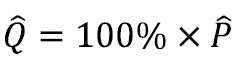 (where P is the proportion and Q is its corresponding percent), then
  .
.Note the difference between the formulas to approximate the standard error for proportions and ratios - the plus sign in the ratio formula has been replaced with a minus sign in proportions formula. If the value under the square root sign is negative, use the ratio standard error formula instead.
If Z > 1.645 or Z < -1.645, then the difference can be said to be statistically significant at the 90 percent confidence level.1 Any estimate can be compared to a PRCS estimate using this method, including other PRCS estimates from the current year, the PRCS estimate for the same characteristic and geographic area but from a previous year, ACS estimates, Census 2000 100 percent counts and long form estimates, estimates from other Census Bureau surveys, and estimates from other sources. Not all estimates have sampling error - Census 2000 100 percent counts do not, for example, although Census 2000 long form estimates do - but they should be used if they exist to give the most accurate result of the test.
Users are also cautioned to not rely on looking at whether confidence intervals for two estimates overlap or not to determine statistical significance, because there are circumstances where that method will not give the correct test result. If two confidence intervals do not overlap, then the estimates will be significantly different (i.e. the significance test will always agree). However, if two confidence intervals do overlap, then the estimates may or may not be significantly different. The Z calculation above is recommended in all cases.
Here is a simple example of why it is not recommended to use the overlapping confidence bounds rule of thumb as a substitute for a statistical test.
Let: X1 = 5.0 with SE1 = 0.2 and X2 = 6.0 with SE2 = 0.5.
The Upper Bound for X1 = 5.0 + 0.2 * 1.645 = 5.3 while the Lower Bound for X2 = 6.0 - 0.5 * 1.645 = 5.2. The confidence bounds overlap, so, the rule of thumb would indicate that the estimates are not significantly different at the 90% level.
However, if we apply the statistical significance test we obtain:
Z = 1.857 > 1.645 which means that the difference is significant (at the 90% level).
All statistical testing in PRCS data products is based on the 90 percent confidence level. Users should understand that all testing was done using unrounded estimates and standard errors, and it may not be possible to replicate test results using the rounded estimates and margins of error as published.
Footnote:
1The PRCS Accuracy of the Data was not separate from the ACS Accuracy of the Data in 2005, which used a Z statistic of +/-1.65. Data users should use +/-1.65 for estimates published in 2005 or earlier.
The estimated number of males, never married is 660,765 from summary table B12001 for Puerto Rico for 2009. The margin of error is 7,775. Standard Error = Margin of Error / 1.645 Calculating the standard error using the margin of error, we have: SE(660,765) = 7,775/ 1.645 = 4,727.
Example 2 - Calculating the Standard Error of a Sum or Difference
We are interested in the number of people who have never been married. From Example 1, we know the number of males, never married is 660,765. From summary table B12001 we have the number of females, never married is 589,767 with a margin of error of 9,369. So, the estimated number of people who have never been married is 660,765 + 589,767 = 1,250,532. To calculate the approximate standard error of this sum, we need the standard errors of the two estimates in the sum. We have the standard error for the number of males never married from Example 1 as 4,727. The standard error for the number of females never married is calculated using the margin of error:
SE(589,767) = 9,369 / 1.645 = 5,695.
So using formula (2) for the approximate standard error of a sum or difference we have:
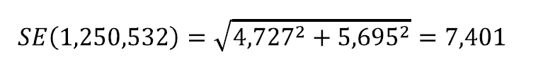
Caution: This method will underestimate or overestimate the standard error if the two estimates interact in either a positive or negative way.
To calculate the lower and upper bounds of the 90 percent confidence interval around 1,250,532 using the standard error, simply multiply 7,401 by 1.645, then add and subtract the product from 1,250,532. Thus the 90 percent confidence interval for this estimate is [1,250,532 - 1.645(7,401)] to [1,250,532 + 1.645(7,401)] or 1,238,357 to 1,262,707.
Example 3 - Calculating the Standard Error of a Proportion/Percent
We are interested in the percentage of females who have never been married to the number of people who have never been married. The number of females, never married is 589,767 and the number of people who have never been married is 1,250,532. To calculate the approximate standard error of this percent, we need the standard errors of the two estimates in the percent. We have the approximate standard error for the number of females never married from Example 2 as 5,695 and the approximate standard error for the number of people never married calculated from example 2 as 7,401.
The estimate is (589,767 / 1,250,532) * 100% = 47.2%
So, using formula (4) for the approximate standard error of a proportion or percent, we have:
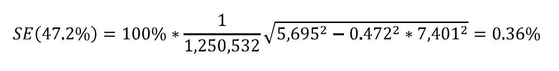
To calculate the lower and upper bounds of the 90 percent confidence interval around 47.2 using the standard error, simply multiply 0.36 by 1.645, then add and subtract the product from 47.2. Thus the 90 percent confidence interval for this estimate is
[47.2 - 1.645(0.36)] to [47.2 + 1.645(0.36)], or 46.6% to 47.8%.
Example 4 - Calculating the Standard Error of a Ratio
Now, let us calculate the estimate of the ratio of the number of unmarried males to the number of unmarried females and its standard error. From the above examples, the estimate for the number of unmarried men is 660,765 with a standard error of 4,727, and the estimates for the number of unmarried women is 589,767 with a standard error of 5,695. The estimate of the ratio is 660,765 / 589,767 = 1.120. Using formula (3) for the approximate standard error we have:
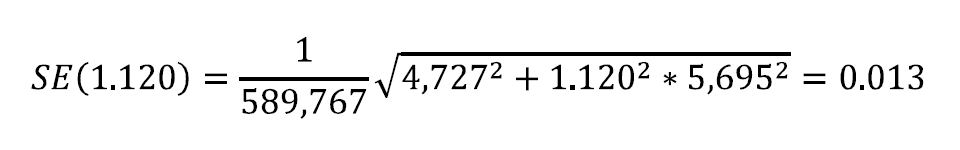
The 90 percent margin of error for this estimate would be 0.013 multiplied by 1.645, or about 0.021. The 90 percent lower and upper 90 percent confidence bounds would then be [1.120- 0.021] to [1.120 + 0.021], or 1.098 and 1.142.
Example 5 - Calculating the Standard Error of a Product
We are interested in the number of 1-unit detached owner-occupied housing units. The number of owner-occupied housing units is 844,860 with a margin of error of 7,873 from subject table S2504 for 2009, and the percent of 1-unit detached owner-occupied housing units is 79.4% (0.794) with a margin of error of 0.5 (0.005). So the number of 1-unit detached owner-occupied housing units is 844,860 * 0.794 = 670,819. Calculating the standard error for the estimates using the margin of error we have:
SE(844,860) = 7,873/1,645 = 4,786
and
SE(0.794) = 0.005/1,645 = 0.0030395
The approximate standard error for number of 1-unit detached owner-occupied housing units is calculated using formula (5) for products as:

To calculate the lower and upper bounds of the 90 percent confidence interval around 670,819 using the standard error, simply multiply 4,586 by 1.645, then add and subtract the product from 670,819. Thus the 90 percent confidence interval for this estimate is
[670,819 - 1.645(4,586)] to [670,819 + 1.645(4,586)] or 663,275 to 678,363.
- Coverage Error - It is possible for some sample housing units or persons to be missed entirely by the survey (undercoverage), but it is also possible for some sample housing units and persons to be counted more than once (overcoverage). Both the undercoverage and overcoverage of persons and housing units can introduce biases into the data, increase respondent burden and survey costs.
A major way to avoid coverage error in a survey is to ensure that its sampling frame, for Puerto Rico an address list in each municipio, is as complete and accurate as possible. The source of addresses for the PRCS is the MAF, which was created using the address list for Census 2000. An attempt is made to assign all appropriate geographic codes to each MAF address via an automated procedure using the Census Bureau TIGER (Topologically Integrated Geographic Encoding and Referencing) files. A manual coding operation based in the appropriate regional offices is attempted for addresses, which could not be automatically coded. The MAF was used as the source of addresses for selecting sample housing units and mailing questionnaires. TIGER produced the location maps for CAPI assignments. Sometimes the MAF has an address that is the duplicate of another address already on the MAF. This could occur when there is a slight difference in the address such as 123 Calle 1, Bayamon versus URB Hermosillo, 123 Calle 1, Bayamon.
In the CATI and CAPI nonresponse follow-up phases, efforts were made to minimize the chances that housing units that were not part of the sample were interviewed in place of units in sample by mistake. If a CATI interviewer called a mail nonresponse case and was not able to reach the exact address, no interview was conducted and the case was eligible for CAPI. During CAPI follow-up, the interviewer had to locate the exact address for each sample housing unit. If the interviewer could not locate the exact sample unit in a multi-unit structure, or found a different number of units than expected, the interviewers were instructed to list the units in the building and follow a specific procedure to select a replacement sample unit. Person overcoverage can occur when an individual is included as a member of a housing unit but does not meet PRCS residency rules.
Coverage rates give a measure of undercoverage or overcoverage of persons or housing units in a given geographic area. Rates below 100 percent indicate undercoverage, while rates above 100 percent indicate overcoverage. Coverage rates are released concurrent with the release of estimates on American FactFinder in the B98 series of detailed tables. Further information about PRCS coverage rates may be found at http://www.census.gov/acs/www/methodology/sample_size_and_data_quality/.
- Nonresponse Error - Survey nonresponse is a well-known source of nonsampling error. There are two types of nonresponse error - unit nonresponse and item nonresponse. Nonresponse errors affect survey estimates to varying levels depending on amount of nonresponse and the extent to which nonrespondents differ from respondents on the characteristics measured by the survey. The exact amount of nonresponse error or bias on an estimate is almost never known. Therefore, survey researchers generally rely on proxy measures, such as the nonresponse rate, to indicate the potential for nonresponse error.
- Unit Nonresponse - Unit nonresponse is the failure to obtain data from housing units in the sample. Unit nonresponse may occur because households are unwilling or unable to participate, or because an interviewer is unable to make contact with a housing unit. Unit nonresponse is problematic when there are systematic or variable differences between interviewed and noninterviewed housing units on the characteristics measured by the survey. Nonresponse bias is introduced into an estimate when differences are systematic, while nonresponse error for an estimate evolves from variable differences between interviewed and noninterviewed households.
The PRCS made every effort to minimize unit nonresponse, and thus, the potential for nonresponse error. First, the PRCS used a combination of mail, CATI, and CAPI data collection modes to maximize response. The mail phase included a series of three to four mailings to encourage housing units to return the questionnaire. Subsequently, mail nonrespondents (for which phone numbers are available) were contacted by CATI for an interview. Finally, a subsample of the mail and telephone nonrespondents was contacted for by personal visit to attempt an interview PRCS response rates measure the percent of units with a completed interview. The higher the response rate, and consequently the lower the nonresponse rate, the less chance estimates may be affected by nonresponse bias. Response and nonresponse rates, as well as rates for specific types of nonresponse, are released concurrent with the release of estimates on American FactFinder in the B98 series of detailed tables. Further information about response and nonresponse rates may be found at http://www.census.gov/acs/www/methodology/sample_size_and_data_quality/.
- Item Nonresponse - Nonresponse to particular questions on the survey questionnaire and instrument allows for the introduction of error or bias into the data, since the characteristics of the nonrespondents have not been observed and may differ from those reported by respondents. As a result, any imputation procedure using respondent data may not completely reflect this difference either at the elemental level (individual person or housing unit) or on average.
Some protection against the introduction of large errors or biases is afforded by minimizing nonresponse. In the PRCS, item nonresponse for the CATI and CAPI operations was minimized by the requirement that the automated instrument receive a response to each question before the next one could be asked. Questionnaires returned by mail were edited for completeness and acceptability. They were reviewed by computer for content omissions and population coverage. If necessary, a telephone follow-up was made to obtain missing information. Potential coverage errors were included in this follow-up.
Allocation tables provide the weighted estimate of persons or housing units for which a value was imputed, as well as the total estimate of persons or housing units that were eligible to answer the question. The smaller the number of imputed responses, the lower the chance that the item nonresponse is contributing a bias to the estimates. Allocation tables are released concurrent with the release of estimates on American Factfinder in the B99 series of detailed tables with the overall allocation rates across all person and housing unit characteristics in the B98 series of detailed tables.
Additional information on item nonresponse and allocations can be found at http://www.census.gov/acs/www/methodology/sample_size_and_data_quality/.
- Measurement and Processing Error - The person completing the questionnaire or responding to the questions posed by an interviewer could serve as a source of error, although the questions were cognitively tested for phrasing, and detailed instructions for completing the questionnaire were provided to each household.
- Interviewer monitoring - The interviewer may misinterpret or otherwise incorrectly enter information given by a respondent; may fail to collect some of the information for a person or household; or may collect data for households that were not designated as part of the sample. To control these problems, the work of interviewers was monitored carefully. Field staff were prepared for their tasks by using specially developed training packages that included hands-on experience in using survey materials. A sample of the households interviewed by CAPI interviewers was reinterviewed to control for the possibility that interviewers may have fabricated data.
- Processing Error - The many phases involved in processing the survey data represent potential sources for the introduction of nonsampling error. The processing of the survey questionnaires includes the keying of data from completed questionnaires, automated clerical review, follow-up by telephone, manual coding of write-in responses, and automated data processing. The various field, coding and computer operations undergo a number of quality control checks to insure their accurate application.
- Content Editing - After data collection was completed, any remaining incomplete or inconsistent information was imputed during the final content edit of the collected data. Imputations, or computer assignments of acceptable codes in place of unacceptable entries or blanks, were needed most often when an entry for a given item was missing or when the information reported for a person or housing unit on that item was inconsistent with other information for that same person or housing unit. As in other surveys and previous censuses, the general procedure for changing unacceptable entries was to allocate an entry for a person or housing unit that was consistent with entries for persons or housing units with similar characteristics. Imputing acceptable values in place of blanks or unacceptable entries enhances the usefulness of the data.
Table A: 2009 Estimates of males from B05003: Sex by Age by Citizenship Status
| Characteristic | Estimate | MOE |
|---|---|---|
| Male | 1,905,314 | 2,996 |
| Under 18 Years | 493,406 | 2,300 |
| Native | 491,306 | 2,312 |
| Foreign Born | 2,100 | 697 |
| Naturalized U.S. Citizen | 94 | 163 |
| Not a U.S. Citizen | 2,006 | 687 |
| 18 Years and Older | 1,411,908 | 1,572 |
| Native | 1,363,983 | 4,197 |
| Foreign Born | 47,925 | 4,108 |
| Naturalized U.S. Citizen | 19,549 | 2,150 |
| Not a U.S. Citizen | 28,376 | 3,290 |
2009 American FactFinder
The estimate and its MOE are actually published. However, if they were not available in the tables, one way of obtaining them would be to add together the number of males under 18 and over 18 to get:
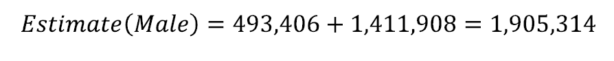
And the first approximated
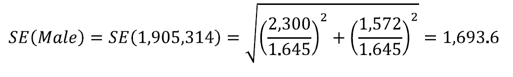
Another way would be to add up the estimates for the three subcategories (Native, Foreign Born: Naturalized U.S. Citizen, and Foreign Born: Not a U.S. Citizen), for males under and over 18 years of age. From these eight estimates we obtain:
Estimate(Male) = 491,306 + 94 + 2,006 + 1,363,983 + 19,549 + 28,376 = 1,905,314
With a second approximation to the SE of:
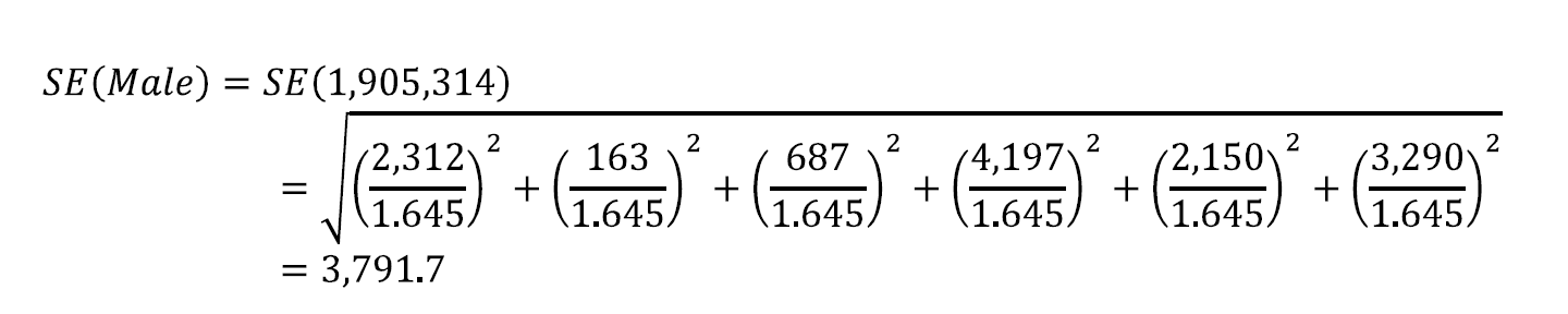
We do know that the standard error using the published MOE is 2,996 / 1.645 = 1,821.3. With a quick glance, we can see that the ratio of the standard error of the first method to the published-based standard error yields 0.93; an under-estimate of roughly 7%, whereas the second method yields a ratio of 2.08 or an over-estimate of 108%. This is an example of what could happen to the approximate SE when the sum involves a controlled estimate. In this case, it is sex by age.
B. Suppose we are interested in the total number of people aged 65 or older and its standard error. Table B shows some of the estimates for the national level from table B01001 (the estimates in gray were derived for the purpose of this example only).
Table B: Some Estimates from AFF Table B01001: Sex by Age for 2009
| Age Category | Estimate, Male | MOE, Male | Estimate, Female | MOE, Female | Total | Estimated MOE, Total |
|---|---|---|---|---|---|---|
| 65 and 66 years old | 34,387 | 2,210 | 44,262 | 2,719 | 78,649 | 3,504 |
| 67 to 69 years old | 47,639 | 2,418 | 51,547 | 2,511 | 99,186 | 3,486 |
| 70 to 74 years old | 58,924 | 2,576 | 77,508 | 3,335 | 136,432 | 4,214 |
| 75 to 79 years old | 42,091 | 1,912 | 58,788 | 2,639 | 100,879 | 3,259 |
| 80 to 84 years old | 31,494 | 2,237 | 41,300 | 2,418 | 72,794 | 3,294 |
| 85 years and older | 26,399 | 1,790 | 45,063 | 2,595 | 71,462 | 3,152 |
| Total | 240,934 | NA | 318,468 | NA | 559,402 | 8,579 |
To begin we find the total number of people aged 65 and over by simply adding the totals for males and females to get 240,934 + 318,468 = 559,402. One way we could approximate the standard error of this estimate is to sum the males and females for each age category and then use their MOEs to obtain the approximate standard error for the total number of people over 65.
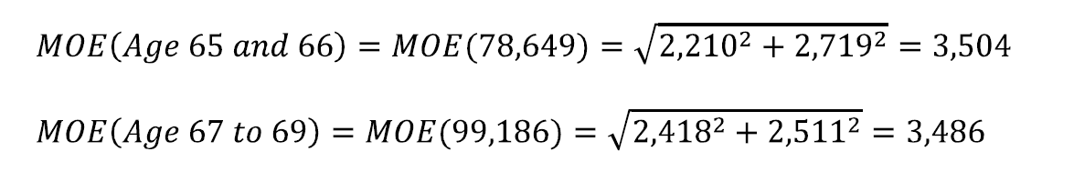
... etc ...
Now, we calculate the number of people aged 65 or older, 559,402, using the six derived estimates and approximate its standard error:
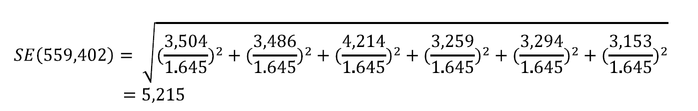
For this example the estimate and MOE are published in table B09017. The total number of people aged 65 or older is 559,402 with a margin of error of 2,595. Therefore the published-based standard error is:
SE(559,402) = 2,595/1.645 = 1,578
The approximated standard error, using the six derived age group estimates, yields an approximated standard error roughly 3.3 times larger than the published-based standard error.
There are two additional ways to approximate the standard error of people aged 65 and over in addition to the way used above. The first is to find the MOEs for the males age 65 and older, and females aged 65 and older separately and then combine them to find the approximated standard error.
For males it is:

And for females:

And the total is then:
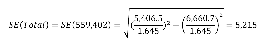
The second is to use all twelve of the published estimates together, that is, all estimates from the male age categories and female age categories, to create the SE for people aged 65 and older.

And the standard error is:
SE(Total) = SE(559,402) = 8,578.8/1.645 = 5,215
In this particular situation, the results from all three ways are the same. So no matter which way you use, you will obtain the same approximation for the standard error. This is not always the case. The corresponding section in the ACS Accuracy of the Data document gives an example where the three methods yield different answers. It is located at http://www.census.gov/acs/www/data_documentation/documentation_main/.
C. For an alternative to approximating the standard error for people 65 years and older seen in part B, we could find the estimate and its SE by summing all of the estimate for the ages less than 65 years old and subtracting them from the estimate for the total population. Due to the large number of estimates, the Table C does not show all of the age groups. In addition, the estimates in the part of the table shaded gray were derived for the purposes of this example only and cannot be found in base table B01001.
Table C: Some Estimates from AFF Table B01001: Sex by Age for 2009:
| Age Category | Estimate, Male | MOE, Male | Estimate, Female | MOE, Female | Total | Estimated MOE, Total |
|---|---|---|---|---|---|---|
| Total Population | 1,905,314 | 2,996 | 2,061,974 | 2,996 | 3,967,288 | 4,237 |
| Under 5 years | 119,417 | 1,668 | 114,240 | 1,654 | 233,657 | 2,349 |
| 5 to 9 years old | 132,539 | 4,060 | 118,361 | 3,987 | 250,900 | 5,690 |
| 10 to 14 years old | 150,027 | 4,079 | 150,448 | 4,085 | 300,475 | 5,773 |
| ... | ... | ... | ... | ... | ... | ... |
| 62 to 64 years old | 61,327 | 3,232 | 73,135 | 3,368 | 134,462 | 4,668 |
| Total for Age 0 to 64 years old | 1,664,380 | 11,945 | 1,743,506 | 12,948 | 3,407,886 | 17,617 |
| Total for Age 65 years and older | 240,934 | 12,315 | 318,468 | 13,290 | 559,402 | 18,119 |
An estimate for the number of people age 65 and older is equal to the total population minus the population between the ages of zero and 64 years old:Number of people aged 65 and older: 3,967,288 - 3,407,886 = 559,402. The way to approximate the SE is the same as in part B. First we will sum males and females estimates across each age category and then approximate the MOEs. We will use that information to approximate the standard error for our estimate of interest:
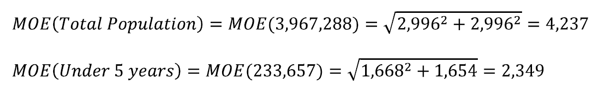
... etc ...
And the SE for the total number of people aged 65 and older is:
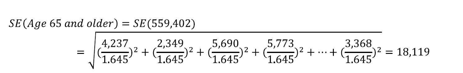
Again, as in Example B, the estimate and its MOE are published in table B09017. The total number of people aged 65 or older is 559,402 with a margin of error of 2,595. Therefore the standard error is:
SE(559,402) = 2,595 / 1.645 = 1,578.
The approximated standard error using the thirteen derived age group estimates yields a standard error roughly 11.5 times larger than the actual SE.
Data users can mitigate the problems shown in examples A through C to some extent by using a collapsed version of a detailed table if available which will reduce the number of estimates and SEs. These issues may also be avoided by creating estimates and SEs using the Public Use Microdata Sample (PUMS) or by requesting a custom tabulation, a fee-based service offered under certain conditions by the Census Bureau. More information regarding custom tabulations may be found at http://www.census.gov/acs/www/data_documentation/custom_tabulations/.
1. ACS data from published tables on American FactFinder
All ACS estimates from tables on AFF include either the 90 percent margin of error or 90 percent confidence bounds. The margin of error is the maximum difference between the estimate and the upper and lower confidence bounds. Most tables on AFF containing 2005 or later ACS data display the margin of error.
Use the margin of error to calculate the standard error (dropping the +/- from the displayed value first) as:
Standard Error = Margin of Error / Z
where Z = 1.645 for 2006 ACS data and recent years. Users of 2005 and earlier ACS data should use Z= 1.65
If confidence bounds are provided instead (as with most ACS data products for 2004 and earlier), calculate the margin of error first before calculating the standard error:
Margin of Error = max (upper bound - estimate, estimate - lower bound)
All published ACS estimates use 1.645 (for 2006 and recent years) to calculate 90 percent margins of error and confidence bounds. ACS estimates for years earlier than 2006 should use 1.65. Other surveys may use other values.
2. ACS public-use microdata sample (PUMS) tabulations
Using the methods described in the Accuracy of the PUMS documentation users can calculate standard errors for their tabulations using a design factor method or a replicate weight method. For example, 2008 Accuracy of the PUMS documentation can be used with the 2008 ACS PUMS file to calculate standard errors. This document is available under Data and Documentation on the ACS website (www.census.gov/acs).
NOTE: ACS PUMS design factors provided in the Accuracy of the PUMS document should not be used to calculate standard errors of full ACS sample estimates, such as those found in data tables on AFF. In addition, Census 2000 design factors should not be used to calculate standard errors for any ACS estimate.
All methods in this section are approximations and users should be cautious in using them. This is because these methods do not consider the correlation or covariance between the basic estimates. They may be overestimates or underestimates of the derived estimates standard error depending on whether the two basic estimates are highly correlated in either the positive or negative direction. As a result, the approximated standard error may not match direct calculations of standard errors or calculations obtained through other methods.
- Sum or Difference of Estimates
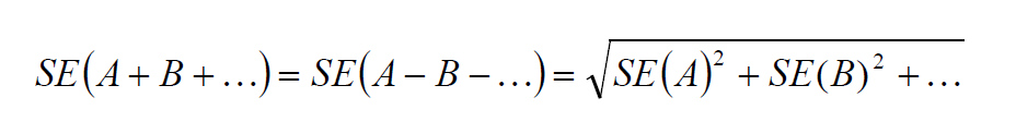
As the number of basic estimates involved in the sum or difference increases, the results of this formula become increasingly different from the standard error derived directly from the ACS microdata. Care should be taken to work with the fewest number of basic estimates as possible. If there are estimates involved in the sum that are controlled in the weighting then the approximate standard error can be tremendously different.
- Proportions and Percents
Here we define a proportion as a ratio where the numerator is a subset of the denominator, for example the proportion of persons 25 and over with a high school diploma or higher.
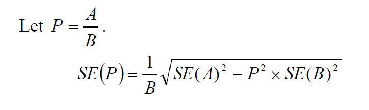
If the value under the square root sign is negative, then instead use
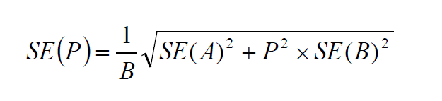
If P =1 then use
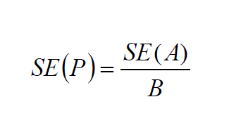
If Q = 100% x P (a percent instead of a proportion), then SE(Q) = 100% x SE(P).
- Means and Other Ratios
If the estimate is a ratio but the numerator is not a subset of the denominator, such as persons per household, per capita income, or percent change, then
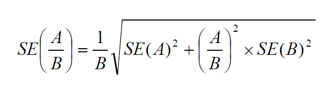
- Products
For a product of two estimates - for example if users want to estimate a proportions numerator by multiplying the proportion by its denominator - the standard error can be approximated as
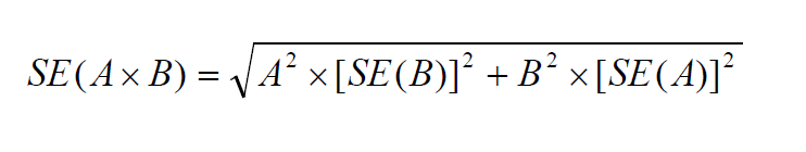
Users may combine these procedures for complicated estimates. For example, if the desired estimate is
then SE(A+B+C) and SE(D+E) can be estimated first, and then those results used to calculate SE(P). For examples of these formulas, please see any "Accuracy of the Data" document under "Data and Documentation" on the ACS website (www.census.gov/acs). The 2009 Accuracy of the Data will be available September 28, 2010.
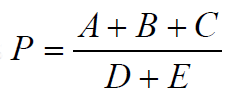 .
.If Z < -1.645 or Z > 1.645, then the difference between A and B is significant at the 90 percent confidence level. Otherwise, the difference is not significant. This means that there is less than a 10 percent chance that the difference between these two estimates would be as large or larger by random chance alone.
Users may choose to apply a confidence level different from 90 percent to their tests of statistical significance. For example, if Z < -1.96 or Z > 1.96, then the difference between A and B is significant at the 95 percent confidence level.
This method can be used for any types of estimates: counts, percentages, proportions, means, medians, etc. It can be used for comparing across years, or across surveys. If one of the estimates is a fixed value or comes from a source without sampling error (such as the Census 2000 SF1), use zero for the standard error for that estimate in the above equation for Z. NOTE: Making comparisons between ACS single-year and multiyear estimates is very difficult, but can be done with caution. Instructions for applying statistical testing to ACS Multiyear data are forthcoming under Data and Documentation on the ACS website (www.census.gov/acs).
This is the method used in determining statistical significance for the ACS Ranking Tables published on AFF. Note that the users determination of statistical significance may not match the Ranking Tables result for the same pair of estimates, because the significance tests for the Ranking Tables are made using unrounded standard errors. Standard errors obtained from the rounded margins of error or confidence bounds are unlikely to match the unrounded standard error, and so statistical tests may differ.
Using the rule of thumb of overlapping confidence intervals does not constitute a valid significance test and users are discouraged from using that method.

